# Load packages
library(GAMBLR.open)
library(dplyr)Tutorial: The prettiest oncoplot
One of the main features and integral parts of this package is the display of coding mutations across a set of genes in a given cohort. Because it outperforms other tools and generates display items with a lot of supported features and flexibility, it is called prettyOncoplot and it belongs to the pretty family of GAMBLR.viz functions. This tutorial will demonstate how to prepare inputs for it (spoiler alert: no specific formatting is necessary) and what is the format of metadata expected by prettyOncoplot (spoiler alert: just Tumor_Sample_Barcode column and column for any annotation you want to display).
Prepare setup
We will first import the necessary packages:
Next, we will get some data to display. The metadata is expected to be a data frame with one required column: Tumor_Sample_Barcode and any other optional column that you want to display as annotation track. In this example, we will use as example the data set and variant calls from the study that identified genetic subgroup of Follicular lymphoma (FL) associated with histologic transformation to DLBCL.
metadata <- get_gambl_metadata() %>%
    filter(cohort == "FL_Dreval")
Next, we will obtain the coding mutations that will be used in the plotting. The data is a data frame in a standartized maf format.
maf <- get_ssm_by_samples(
    these_samples_metadata = metadata,
    tool_name = "publication"
)

# How does it look like?
dim(maf)
[1] 44777 49head(maf) %>%
select(
Tumor_Sample_Barcode,
Hugo_Symbol,
Variant_Classification
)genomic_data Object
Genome Build: grch37
Showing first 10 rows:
Tumor_Sample_Barcode Hugo_Symbol Variant_Classification
1 FL1001T1 AIFM1 Nonsense_Mutation
2 FL1001T1 USP24 Missense_Mutation
3 FL1001T1 LYST Splice_Site
4 FL1001T1 GCKR Missense_Mutation
5 FL1001T1 ORMDL1 Missense_Mutation
6 FL1001T1 BCL6 Missense_Mutation
Did you know?
You do not have to subset your maf data frame to coding mutations only before using it with the prettyOncoplot. Much like other tools, it will be automatically handled for you to only display coding mutations.
Now we have our metadata and mutations we want to explore, so we are ready to start visualizing the data.
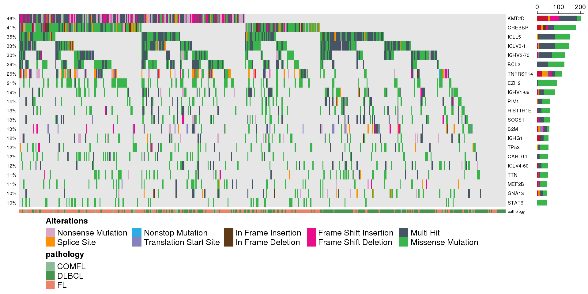
The simplest oncoplot
There is a number of options how to customize your oncoplot, but it is ready for you to use with just the metadata and maf. Here is an example of the output with all default parameters:
minMutationPercent <- 10 # only show genes mutated in at least 10% of samples
prettyOncoplot(
    these_samples_metadata = metadata,
    maf_df = maf,
    minMutationPercent = minMutationPercent
)
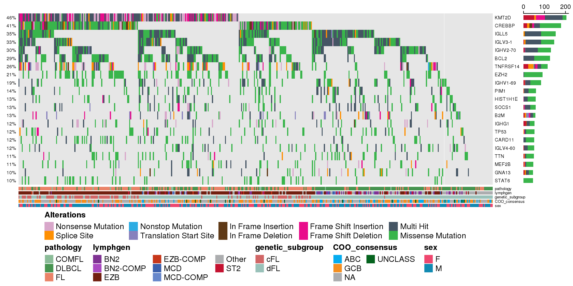
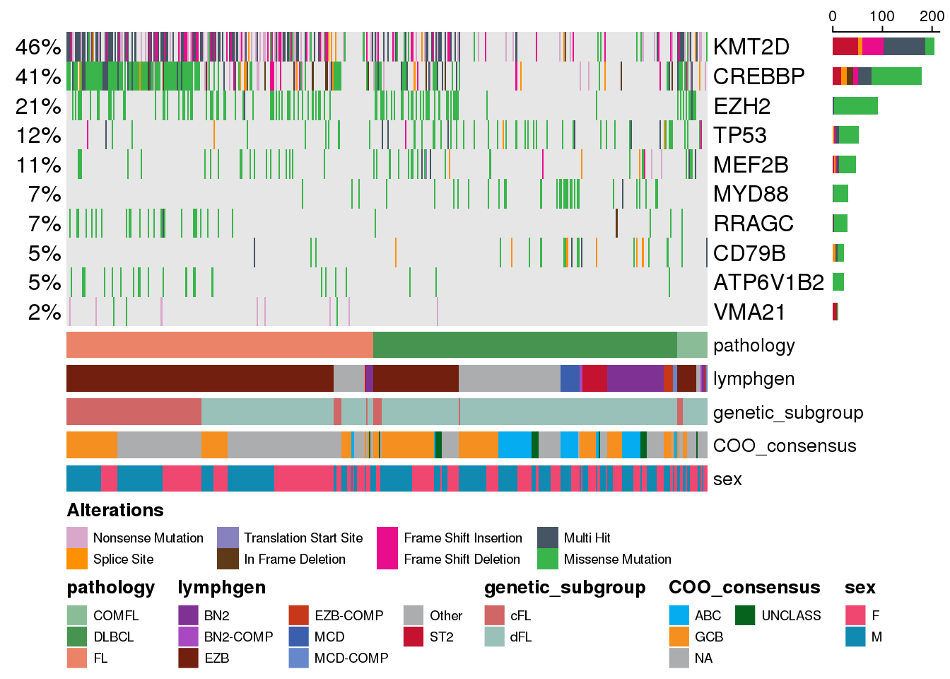
Adding annotation tracks
We can customize this and add some of the annotation tracks for more informative display of the metadata we ate interested in:
metadataColumns <- c(
    "pathology",
    "lymphgen",
    "genetic_subgroup",
    "COO_consensus",
    "sex"
)
prettyOncoplot(
    these_samples_metadata = metadata,
    maf_df = maf,
    minMutationPercent = minMutationPercent,
    metadataColumns = metadataColumns
)
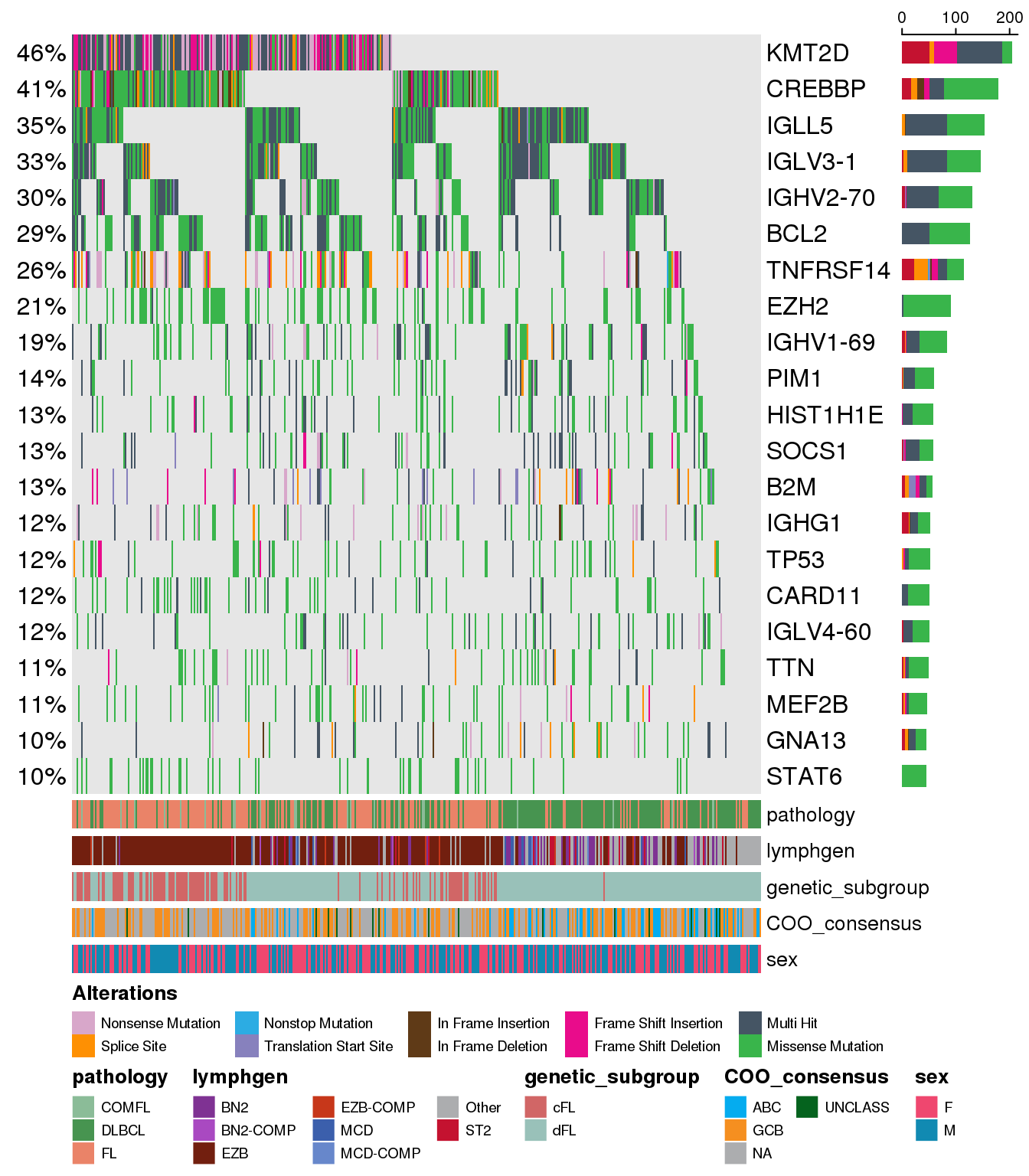
Changing font sizes
You may notice that as more (or less) genes and annotations are displayed with the oncoplot we may want to modify the size of the gene names and/or the annotation tracks with their labels. There are several parameters available for you to do so: - metadataBarHeight: will change the height of the annotation tracks at the bottom of the oncoplot - metadataBarFontsize: will change the font size of the annotation tracks at the bottom of the oncoplot - fontSizeGene: will change the font size of both percentage labels to the right of the oncoplot and gene names to the left of it - legendFontSize: will change the font size of the legend at the bottom of the plot Let’s see these parameters in action:
metadataBarHeight <- 5
metadataBarFontsize <- 10
fontSizeGene <- 12
legendFontSize <- 7

prettyOncoplot(
    these_samples_metadata = metadata,
    maf_df = maf,
    minMutationPercent = minMutationPercent,
    metadataColumns = metadataColumns,
    metadataBarHeight = metadataBarHeight,
    metadataBarFontsize = metadataBarFontsize,
    fontSizeGene = fontSizeGene,
    legendFontSize = legendFontSize
)
Show samples ordered on annotations
We can notice that the default setting generates the classic “rainfall” style of the plot - but what if we want to add some structure to it and sort sample order in some way? It is easy to do so with the parameter sortByColumns. We can sort on the same annotations as we use to display with the oncoplot:
prettyOncoplot(
    these_samples_metadata = metadata,
    maf_df = maf,
    minMutationPercent = minMutationPercent,
    metadataColumns = metadataColumns,
    metadataBarHeight = metadataBarHeight,
    metadataBarFontsize = metadataBarFontsize,
    fontSizeGene = fontSizeGene,
    legendFontSize = legendFontSize,
    sortByColumns = metadataColumns
)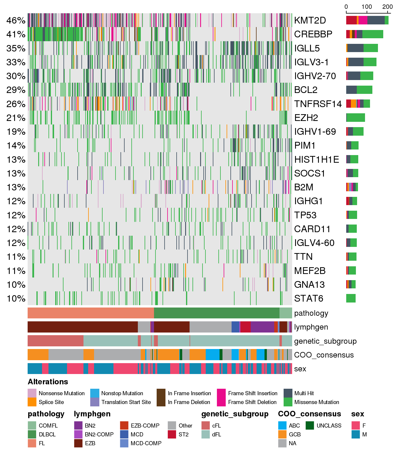
Did you know?
The ordering occurs sequentially according to the order of individual columns we have specified with the sortByColumns parameter. The ordering is in ascending order, and can be toggled with additional boolean parameter arrange_descending.
Displaying only specific genes
There can be scenarion where we might want to diplay genes not based on their recurrence, but out of interest in specific genes. Sure so, one way to do it is to pre-filter your maf data to the genes of interest. But this might have some unexpected consequences and limit your flexibility in doing more things, so the better way is to take advantage of the genes parameter:
fl_genes <- c("RRAGC", "CREBBP", "VMA21", "ATP6V1B2", "EZH2", "KMT2D")
dlbcl_genes <- c("MEF2B", "CD79B", "MYD88", "TP53")
genes <- c(fl_genes, dlbcl_genes)

prettyOncoplot(
    these_samples_metadata = metadata,
    maf_df = maf,
    metadataColumns = metadataColumns,
    metadataBarHeight = metadataBarHeight,
    metadataBarFontsize = metadataBarFontsize,
    fontSizeGene = fontSizeGene,
    legendFontSize = legendFontSize,
    sortByColumns = metadataColumns,
    genes = genes
)
Note
Note that we removed the minMutationPercent in the last function call since we wanted to see the genes that we specifically requested.
Now we are only looking at some specific genes of interest but they are arranged in the decreasing order of their recurrence in this cohort. What if we want to enforce the gene order on the oncoplot to be exactly the same as we specified it in our gene variable? We can take advantage of the keepGeneOrder parameter:
prettyOncoplot(
    these_samples_metadata = metadata,
    maf_df = maf,
    metadataColumns = metadataColumns,
    metadataBarHeight = metadataBarHeight,
    metadataBarFontsize = metadataBarFontsize,
    fontSizeGene = fontSizeGene,
    legendFontSize = legendFontSize,
    sortByColumns = metadataColumns,
    genes = genes,
    keepGeneOrder = TRUE
)
[1] "RRAGC" "CREBBP" "VMA21" "ATP6V1B2" "EZH2" "KMT2D"
[7] "MEF2B" "CD79B" "MYD88" "TP53" 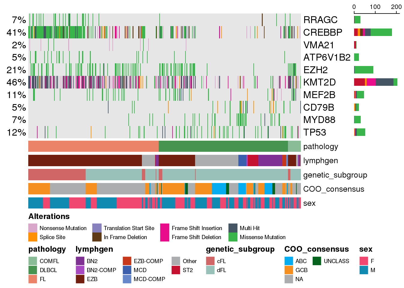
Grouping genes into categories
We can also group genes into specific categories. To do so, we need to have a named list where name of the list element corresponds to the gene name, and the list element corresponds to the gene group. We alreade have the genes variable, so we can convert it to the appropriate format:
gene_groups <- c(
    rep("FL", length(fl_genes)),
    rep("DLBCL", length(dlbcl_genes))
)
names(gene_groups) <- genes

gene_groups
RRAGC CREBBP VMA21 ATP6V1B2 EZH2 KMT2D MEF2B CD79B
"FL" "FL" "FL" "FL" "FL" "FL" "DLBCL" "DLBCL"
MYD88 TP53
"DLBCL" "DLBCL" Now we can use it to split the genes on the oncoplot into the groups:
prettyOncoplot(
    these_samples_metadata = metadata,
    maf_df = maf,
    metadataColumns = metadataColumns,
    metadataBarHeight = metadataBarHeight,
    metadataBarFontsize = metadataBarFontsize,
    fontSizeGene = fontSizeGene,
    legendFontSize = legendFontSize,
    sortByColumns = metadataColumns,
    genes = genes,
    splitGeneGroups = gene_groups
)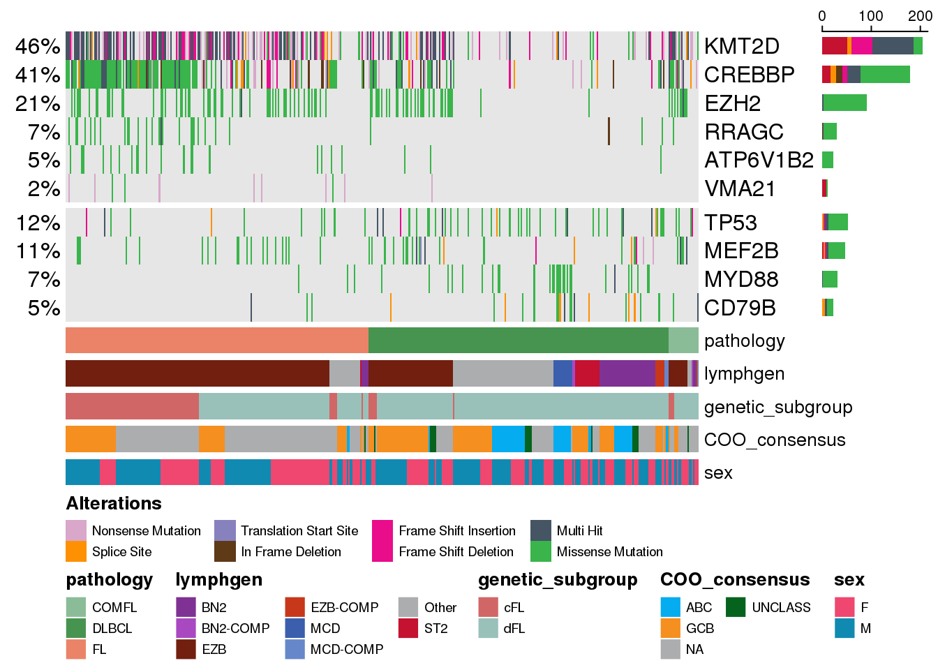
Did you know?
You can provide more than two groups of genes - any number of groups is supported as long as they are specified in the gene_groups.
Note
Within each group, the genes are ordered in decreasing order of their recurrence, but the keepGeneOrder parameter is still supported and if specified, will keep the specified order within each group.
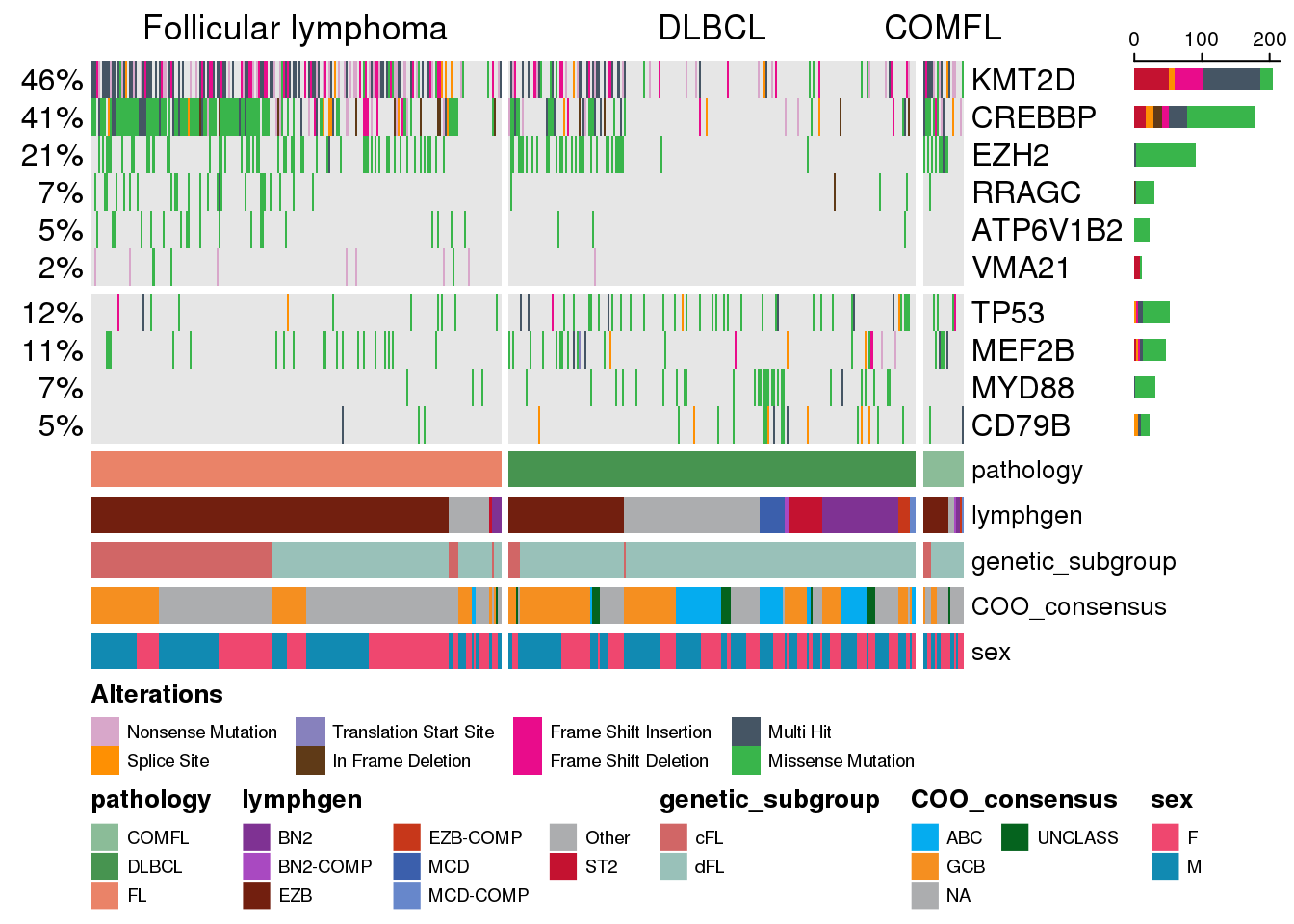
Grouping samples into categories
Similar to the grouping of genes, we can also group samples into certain categories. Typically, it is done based on one of the annotations tracks. By default, there will be no labels for each sample category, but we also have an option of specifying these labels:
prettyOncoplot(
    these_samples_metadata = metadata,
    maf_df = maf,
    metadataColumns = metadataColumns,
    metadataBarHeight = metadataBarHeight,
    metadataBarFontsize = metadataBarFontsize,
    fontSizeGene = fontSizeGene,
    legendFontSize = legendFontSize,
    sortByColumns = metadataColumns,
    genes = genes,
    splitGeneGroups = gene_groups,
    splitColumnName = "pathology",
    groupNames = c("Follicular lymphoma", "DLBCL", "COMFL")
)
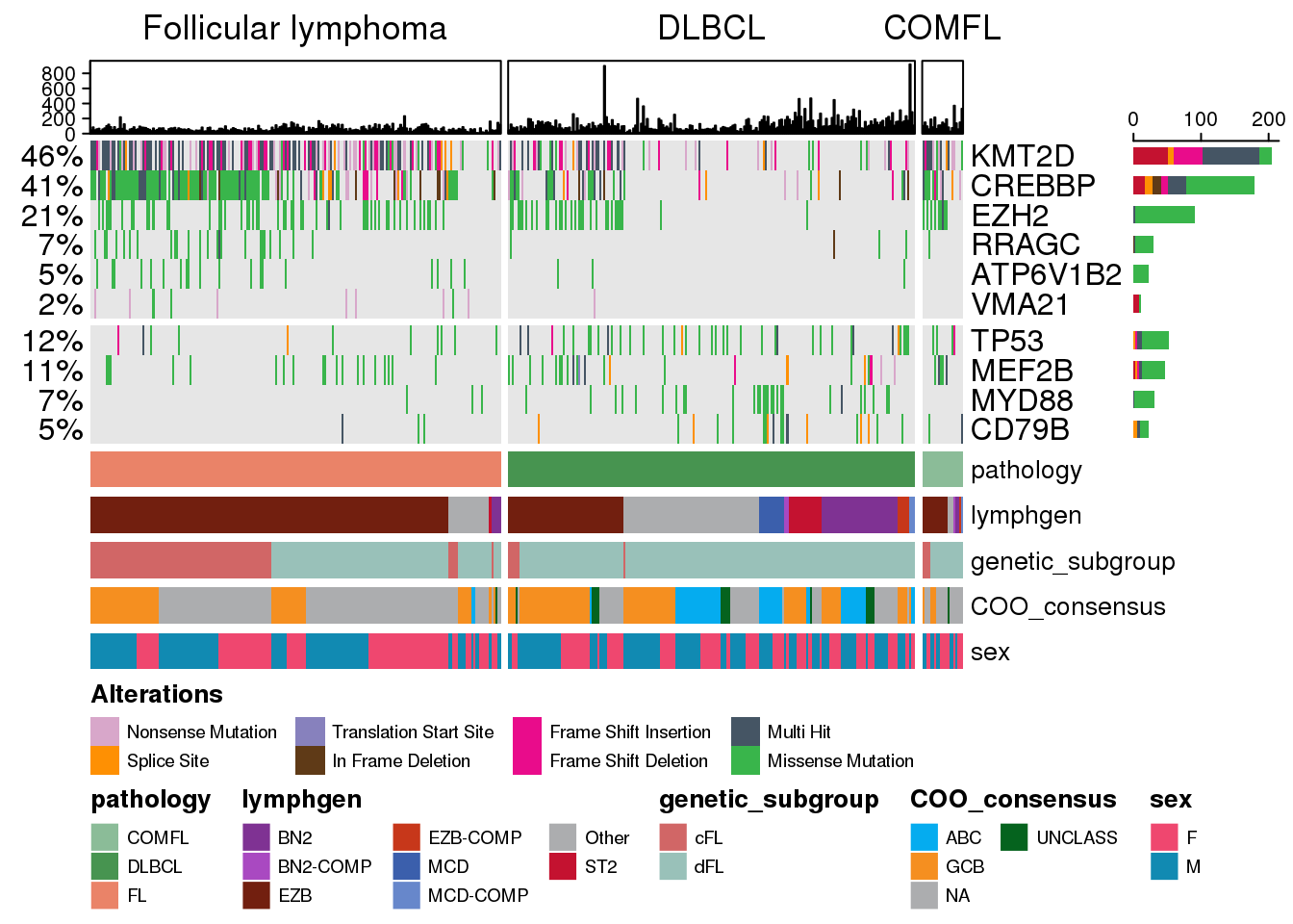
Tallying mutation burden
Previously, we noted that the maf data we were supplying to the prettyOncoplot was not subset to contain only coding mutations, and also discouraged from pre-filtering maf to a subset of genes if we are insterested only looking at some of them. Here is why this is important: if we want to layer on additional information like total mutation burden per sample, any subsetting or filtering of the maf would generate inaccurate and misleading results. Therefore, prettyOncoplot handles all of this for you! So if we were to go ahead with tallying the total mutation burden, we could just add some additional parameters to the function call:
hideTopBarplot <- FALSE # will display TMB annotations at the top
tally_all_mutations <- TRUE # will tally all mutations per sample

prettyOncoplot(
    these_samples_metadata = metadata,
    maf_df = maf,
    metadataColumns = metadataColumns,
    metadataBarHeight = metadataBarHeight,
    metadataBarFontsize = metadataBarFontsize,
    fontSizeGene = fontSizeGene,
    legendFontSize = legendFontSize,
    sortByColumns = metadataColumns,
    genes = genes,
    splitGeneGroups = gene_groups,
    splitColumnName = "pathology",
    groupNames = c("Follicular lymphoma", "DLBCL", "COMFL"),
    hideTopBarplot = hideTopBarplot,
    tally_all_mutations = tally_all_mutations
)
Did you know?
If the dynamic range of total mutation burden is too big and there are some extreme outliers, the bar chart at the top of the oncoplot can be capped of at any numeric value by providing tally_all_mutations_max parameter.
What if we want to additionally force the ordering based on the total number of mutations, so they are nicely arranged in the decreasing order? We can do so by adding the mutation counts as one of the annotation tracks and using it to sort the samples:
# Count all muts to define the order of samples
total_mut_burden <- maf %>%
    count(Tumor_Sample_Barcode)

head(total_mut_burden)
genomic_data Object
Genome Build: grch37
Showing first 10 rows:
Tumor_Sample_Barcode n
1 01-20260T 71
2 02-13135T 98
3 02-20170T 67
4 02-22991T 53
5 03-34157T 26
6 04-24937T 146# Add this info to metadata
metadata <- left_join(
metadata,
total_mut_burden
)
prettyOncoplot(
these_samples_metadata = metadata,
maf_df = maf,
metadataColumns = metadataColumns,
metadataBarHeight = metadataBarHeight,
metadataBarFontsize = metadataBarFontsize,
fontSizeGene = fontSizeGene,
legendFontSize = legendFontSize,
sortByColumns = c("n", metadataColumns),
genes = genes,
splitGeneGroups = gene_groups,
splitColumnName = "pathology",
groupNames = c("Follicular lymphoma", "DLBCL", "COMFL"),
hideTopBarplot = hideTopBarplot,
tally_all_mutations = tally_all_mutations,
numericMetadataColumns = "n",
arrange_descending = TRUE
)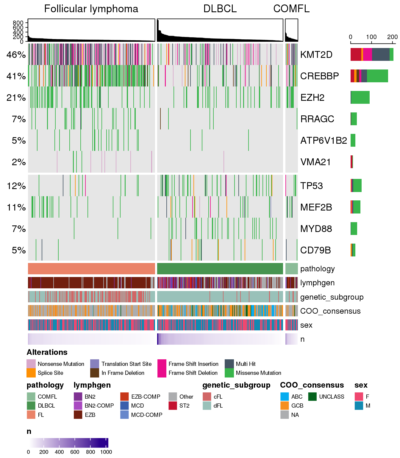
Note
We have modified here the sortByColumns parameter, and provided two additional parameters numericMetadataColumns and arrange_descending.
Did you know?
The top annotation and n annotation at the bottom are the same thing? Remove n from the legend by adding hide_annotations = "n" and remove display of annotation track while keeping the ordering by adding hide_annotations_tracks = TRUE.
Annotating significance of mutation frequencies in sample groups
When looking at our sample plots, we can notice that the frequency of mutations in RRAGC, ATP6V1B2, VMA21 and others is different between FL and DLBCL. But is this difference significant? Can we layer on this diffenerence to the display panel? Yes we can, and this is very easy with GAMBLR family! To do so we will first use another function from GAMBLR.viz to run Fisher’s test and find which genes are significantly different between the FL and DLBCL:
fisher_test <- prettyForestPlot(
    maf = maf,
    metadata = metadata,
    genes = genes,
    comparison_column = "pathology",
    comparison_values = c("DLBCL", "FL"), # we have three pathologies in data
    comparison_name = "FL vs DLBCL"
)
fisher_test$arranged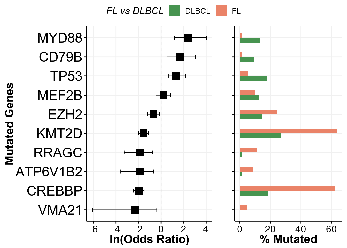
In fact, there are genes that are mutated at significantly different frequencies! Now let’s layer on this information to our oncoplot:
prettyOncoplot(
    these_samples_metadata = metadata,
    maf_df = maf,
    metadataColumns = metadataColumns,
    metadataBarHeight = metadataBarHeight,
    metadataBarFontsize = metadataBarFontsize,
    fontSizeGene = fontSizeGene,
    legendFontSize = legendFontSize,
    sortByColumns = c("n", metadataColumns),
    genes = genes,
    splitGeneGroups = gene_groups,
    splitColumnName = "pathology",
    groupNames = c("Follicular lymphoma", "DLBCL", "COMFL"),
    hideTopBarplot = hideTopBarplot,
    tally_all_mutations = tally_all_mutations,
    numericMetadataColumns = "n",
    arrange_descending = TRUE,
    hide_annotations = "n",
    hide_annotations_tracks = TRUE,
    annotate_specific_genes = TRUE,
    this_forest_object = fisher_test
)
Annotating genes with hotspots
Some genes are mutated at certain positions more often that at others, therefore creating the mutational hotspots - and it we can layer on this level of information to our oncoplot. First, we will need to process our maf data to add a new column called hot_spot which will contain a boolean value showing whether or not particular mutation is a hotspot. If you don’t know how to do it, there is a function for exactly this purpose in the GAMBLR.data, and we will use it in this example:
# Annotate hotspots
maf <- annotate_hotspots(maf)

# What are the hotspots?
maf %>%
    filter(hot_spot) %>%
    select(Hugo_Symbol, hot_spot) %>%
    table()
hot_spot
Hugo_Symbol TRUE
CREBBP 76
EZH2 86
FOXO1 20
MEF2B 23
MYD88 46
STAT6 51
Note
The GAMBLR.data version of the annotate_hotspots only handles very specific genes and does not have functionality to annotate all hotspots.
Now, we can add annotation of the hotspots to the oncoplot display by toggling the highlightHotspots parameter:
highlightHotspots <- TRUE
prettyOncoplot(
    these_samples_metadata = metadata,
    maf_df = maf,
    metadataColumns = metadataColumns,
    metadataBarHeight = metadataBarHeight,
    metadataBarFontsize = metadataBarFontsize,
    fontSizeGene = fontSizeGene,
    legendFontSize = legendFontSize,
    sortByColumns = c("n", metadataColumns),
    genes = genes,
    splitGeneGroups = gene_groups,
    splitColumnName = "pathology",
    groupNames = c("Follicular lymphoma", "DLBCL", "COMFL"),
    hideTopBarplot = hideTopBarplot,
    tally_all_mutations = tally_all_mutations,
    numericMetadataColumns = "n",
    arrange_descending = TRUE,
    hide_annotations = "n",
    hide_annotations_tracks = TRUE,
    annotate_specific_genes = TRUE,
    this_forest_object = fisher_test,
    highlightHotspots = highlightHotspots
)
Co-oncoplot: two plots side-by-side
It may also be informative to generate a display panel where there are two oncoplots displayed side-by-side, so it is possible to visually compare the specific groups of samples while maintaining all annotations and ordering we built so far. For this purpose, the GAMBLR.viz has another function in the pretty family: prettyCoOncoplot. It accepts all of the same parameters as prettyOncoplot with addition of some unique additions. For example, lets break down our sample oncoplot we created so far by the genetic_subgroup and see how cFL compares to dFL:
prettyCoOncoplot(
    metadata = metadata,
    maf = maf,
    comparison_column = "genetic_subgroup",
    label1 = "cFL",
    label2 = "dFL",
    metadataColumns = metadataColumns,
    metadataBarHeight = metadataBarHeight,
    metadataBarFontsize = metadataBarFontsize,
    fontSizeGene = fontSizeGene,
    legendFontSize = legendFontSize,
    sortByColumns = c("n", metadataColumns),
    genes = genes,
    splitGeneGroups = gene_groups,
    splitColumnName = "pathology",
    keepGeneOrder = TRUE,
    groupNames = c("Follicular lymphoma", "DLBCL", "COMFL"),
    hideTopBarplot = hideTopBarplot,
    tally_all_mutations = tally_all_mutations,
    numericMetadataColumns = "n",
    arrange_descending = TRUE,
    hide_annotations = "n",
    hide_annotations_tracks = TRUE,
    annotate_specific_genes = TRUE,
    this_forest_object = fisher_test,
    highlightHotspots = highlightHotspots,
    legend_row = 2,
    annotation_row = 2
)
Note
It is only possible to display two groups side-by-side. If the metadata column you want to split on contains more groups, the specific values can be specified with comparison_values parameter.
Did you know?
Notice that we did not need to create individual maf or metadata objects to supply to prettyCoOncoplot - the same objects we used before are also supported here, but specified with differen parameters metadata and maf.
In the above example, we forced the order of genes to be exaclty as we specified so that the same gene is is displayed on the same row for both oncoplots, othervise they wold not be on the same row due to the different frequencies in each group. In addition to specifying this parameter, we have also enforced specific number of rows in the legend below the plot, so they nicely align between the display items.
Using oncoplot in multi-panel figure
When arranging items for the multi-panel figure when preparing manuscript or experiment report, it may be needed to use the generated oncoplot on the same page as other display items. The prettyOncoplot (and, therefore, prettyCoOncoplot), handles the ComplexHeatmap under the hood to generate graphics, and it is not readily available to be combined with the plots generated with other tools, for example ggplot2. Not readily available - but definitely not impossible! The output of prettyCoOncoplot is directly compatible with the arrangement on multi-panel figure since it uses the trick shown below under the hood to put two panels side-by-side, but the otuput of prettyOncoplot is a ComplexHeatmap object so needs some extra steps to allow multi-panel arrangement. First, lets store the returned oncoplot in a variable:
my_oncoplot <- prettyOncoplot(
    these_samples_metadata = metadata,
    maf_df = maf,
    metadataColumns = metadataColumns,
    metadataBarHeight = metadataBarHeight,
    metadataBarFontsize = metadataBarFontsize,
    fontSizeGene = fontSizeGene,
    legendFontSize = legendFontSize,
    sortByColumns = c("n", metadataColumns),
    genes = genes,
    splitGeneGroups = gene_groups,
    splitColumnName = "pathology",
    groupNames = c("Follicular lymphoma", "DLBCL", "COMFL"),
    hideTopBarplot = hideTopBarplot,
    tally_all_mutations = tally_all_mutations,
    numericMetadataColumns = "n",
    arrange_descending = TRUE,
    hide_annotations = "n",
    hide_annotations_tracks = TRUE,
    annotate_specific_genes = TRUE,
    this_forest_object = fisher_test,
    highlightHotspots = highlightHotspots
)
Next, we will import some of the packages needed to handle the trick:
library(ComplexHeatmap) # to handle the ComplexHeatmap object
library(ggpubr) # to arrange multiple panels
After that, we will capture the display of the oncoplot:
my_oncoplot = grid.grabExpr(
    draw(my_oncoplot),
    width = 10,
    height = 17
)
Now, it is ready for us to arrange in multi-panel figure. We can use the forest plot we already looked at as an example, and put it to the right of the oncoplot:
multipanel_figure <- ggarrange(
    my_oncoplot, # left panel
    fisher_test$arranged, # right panel
    widths = c(1.5, 1), # so the oncoplot is a little wider than the forest
    labels = c("A", "B"), # labels for the panels
    font.label = list( # make labels bold face
        color = "black",
        face = "bold"
    )
)

multipanel_figure
Final note: it would be nice to have the genes in the forest plot directly aligned with the genes as they are displayed on the oncoplot, and we can do this by providing consistent ordering and adding some white space below forest plot to match the height of the oncoplot:
my_oncoplot <- prettyOncoplot(
    these_samples_metadata = metadata,
    maf_df = maf,
    metadataColumns = metadataColumns,
    metadataBarHeight = metadataBarHeight,
    metadataBarFontsize = metadataBarFontsize,
    fontSizeGene = fontSizeGene,
    legendFontSize = legendFontSize,
    sortByColumns = c("n", metadataColumns),
    genes = rev(fisher_test$fisher$gene),
    keepGeneOrder = TRUE,
    splitGeneGroups = gene_groups,
    splitColumnName = "pathology",
    groupNames = c("Follicular lymphoma", "DLBCL", "COMFL"),
    hideTopBarplot = hideTopBarplot,
    tally_all_mutations = tally_all_mutations,
    numericMetadataColumns = "n",
    arrange_descending = TRUE,
    hide_annotations = "n",
    hide_annotations_tracks = TRUE,
    annotate_specific_genes = TRUE,
    this_forest_object = fisher_test,
    highlightHotspots = highlightHotspots
)

my_oncoplot = grid.grabExpr(
    draw(my_oncoplot),
    width = 10,
    height = 17
)

multipanel_figure <- ggarrange(
    my_oncoplot, # left panel
    ggarrange( # right panel
        NULL, # empty space at the top
        fisher_test$arranged, # forest on the top
        NULL, # empty space at the bottom
        nrow = 3, # arrange vertically
        heights = c(0.1, 2.5, 1) # match height of the oncoplot
    ),
    widths = c(1.5, 1), # so the oncoplot is a little wider than the forest
    labels = c("A", "B"), # labels for the panels
    font.label = list( # make labels bold face
        color = "black",
        face = "bold"
    )
)

multipanel_figure