# Load packages
library(GAMBLR.open)
library(tidyverse)Tutorial: Getting started
This is a quick tour of some basic commands and usage patterns, just to get you started.
This tutorial explores how to generate some basic and most common plots, commonly occurring arguments across different functions, best practices and recommendations in the scope of visualizing data.
What are standartized colours?
First, let’s explore the standartized color pallettes in the GAMBLR.viz. They are stored as list in one of the GAMBLR.viz dependencies (GAMBLR.helpers) and are an integral part of visualizations. For demonstration purposes, we will obtain all of the standartized colours:
all_c <- get_gambl_colours(
    as_dataframe = TRUE
)
What are the colours available?
str(all_c)'data.frame': 328 obs. of 3 variables:
$ group : chr "chromosome" "chromosome" "chromosome" "chromosome" ...
$ name : chr "chr1" "chr2" "chr3" "chr4" ...
$ colour: chr "#555FAB" "#CE3D31" "#749B58" "#F0E584" ...What are the colour groups?
table(all_c$group)
       aneuploidy                BL             blood chapuy_classifier
                8                 7                15                 6
       chromosome          clinical            cohort               coo
               23                47                16                12
      copy_number           domains               EBV                FL
               17                24                 4                 3
 genetic_subgroup              hmrn            indels   lacy_classifier
               24                 8                 2                 8
         lymphgen    lymphgenerator          mutation         pathology
               14                10                15                32
          pos_neg          rainfall          seq_type               sex
               13                 7                 3                 6
              svs              type
                2                 2
Many of these colours are conviniently provided for you to ensure consistency that is independent of formatting and case: for example, when the color for DLBCL COO is returned, the same color will be used for UNCLASS, U, UNC, Unclassified etc.
Just for the purpose of this guide, we will define a simple function to display some of these colour pallettes:
show_col <- function(data, group){
    data %>%
        filter(
            !!sym("group") == {{group}}
        ) %>%
        ggplot(
            aes(
                x = name,
                y = 0,
                fill = colour,
                label = name
            )
        ) +
        geom_tile(width = 0.9, height = 1) +
        geom_text(color = "white", fontface="bold") +
        scale_fill_identity(guide = "none") +
        coord_flip() +
        theme_void() +
        labs(title = toupper(group)) +
        theme(plot.title = element_text(lineheight = 0.9,hjust=0.5,face="bold"))
}
Hex codes for B-cell lymphomas
show_col(all_c, "pathology")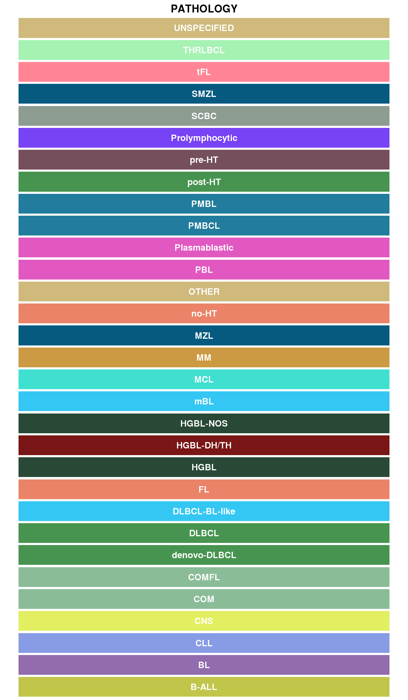
Hex codes for genetic subgroups
show_col(all_c, "genetic_subgroup")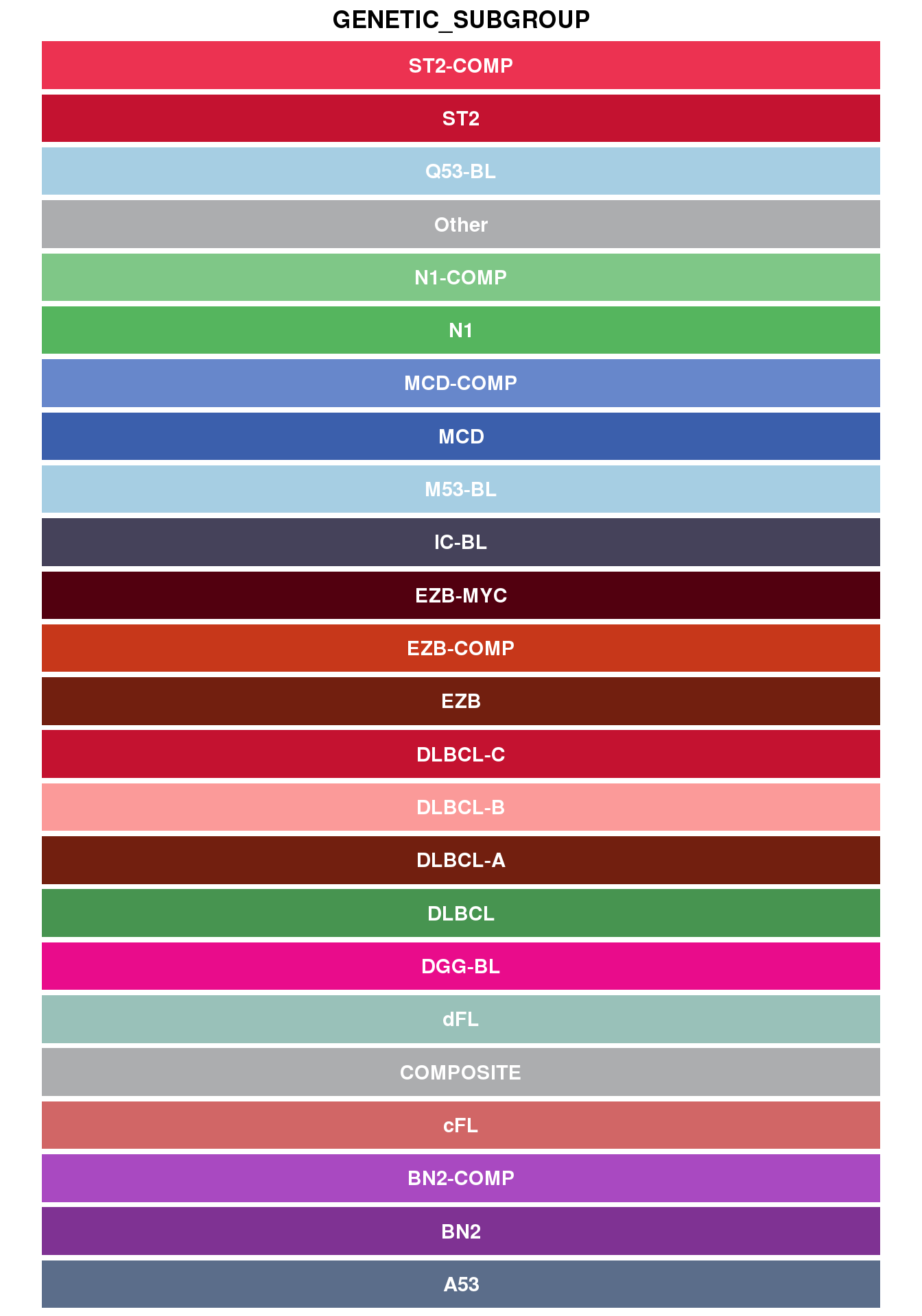
Hex codes for clinical variables
show_col(all_c, "clinical")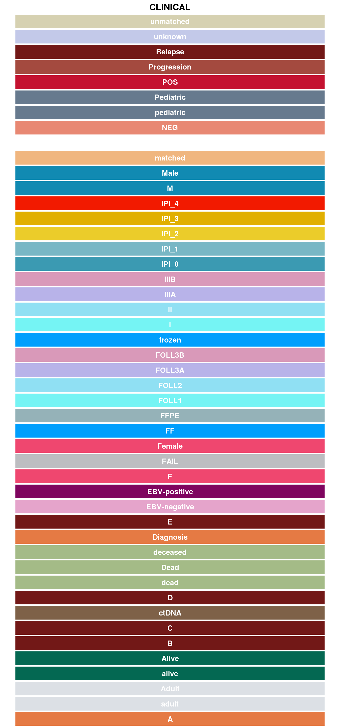
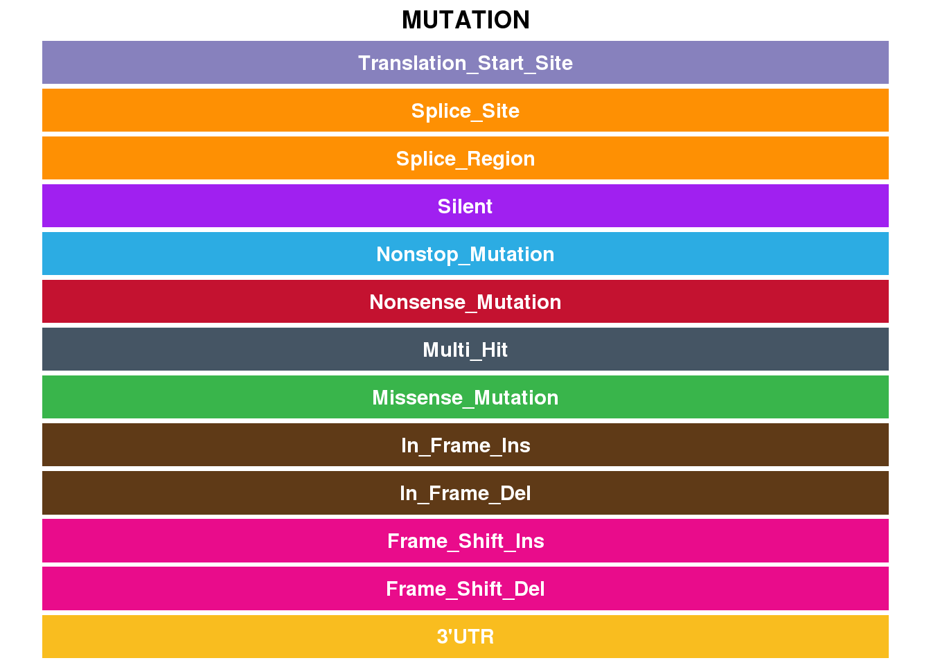
Hex codes for Mutation types
show_col(all_c, "mutation")