DLBCLone: Full Walkthrough • GAMBLR.predict

A step by step example workflow from start to finish

library(GAMBLR.open)
library(tidyverse)

Training data

For simplicity, we’ll skip feature selection and train our new model using a set of genes that have been pre-selected for you based on a model described in the DLBCLone preprint. The code below shows how to infer what features were used in training our model, starting with the column names of the model’s features (model_feats).

SSM features

# Full set of genes considered for SSM

model_genes = grep("_SV|HOTS",model_feats,invert=T,value=T)

model_genes

 [1] "ACTB"     "ACTG1"    "BCL10"    "BCL2"     "BCL2L1"   "BCL6"
 [7] "BIRC3"    "BRAF"     "BTG1"     "BTG2"     "BTK"      "CD19"
[13] "CD70"     "CD79B"    "CD83"     "CDKN2A"   "CREBBP"   "DDX3X"
[19] "DTX1"     "DUSP2"    "EDRF1"    "EIF4A2"   "EP300"    "ETS1"
[25] "ETV6"     "EZH2"     "FAS"      "FCGR2B"   "FOXC1"    "FOXO1"
[31] "GNA13"    "GRHPR"    "HLA-A"    "HLA-B"    "HNRNPD"   "IRF4"
[37] "IRF8"     "ITPKB"    "JUNB"     "KLF2"     "KLHL14"   "KLHL6"
[43] "KMT2D"    "MEF2B"    "MPEG1"    "MYD88"    "NFKBIA"   "NFKBIE"
[49] "NFKBIZ"   "NOL9"     "NOTCH1"   "NOTCH2"   "OSBPL10"  "PIM1"
[55] "PIM2"     "PRDM1"    "PRDM15"   "PRKDC"    "PRRC2C"   "PTPN1"
[61] "RFTN1"    "S1PR2"    "SETD1B"   "SGK1"     "SOCS1"    "SPEN"
[67] "STAT3"    "STAT6"    "TBCC"     "TBL1XR1"  "TET2"     "TMEM30A"
[73] "TMSB4X"   "TNFAIP3"  "TNFRSF14" "TOX"      "TP53"     "TP73"
[79] "UBE2A"    "WEE1"     "XBP1"     "ZFP36L1"

Hotspot features

# Genes with hotspots considered

hotspot_features = grep("HOTS",model_feats,invert=F,value=T) 
hotspot_features

[1] "MYD88HOTSPOT"

SV features

SV_genes = grep("_SV",model_feats,invert=F,value=T)
SV_genes

[1] "BCL2_SV" "BCL6_SV"

Load and subset the training data

The GAMBLR.predict package is bundled with base-3 mutation status matrix for the training data set. The code below shows how to load that into a data frame (setting sample_id as the row names) and subset it to only the features described above.

best_opt_model_matrix <- readr::read_tsv(
  system.file("extdata/all_full_status.tsv",
             package = "GAMBLR.predict")) %>%
  tibble::column_to_rownames("sample_id") 

# keep only the columns you want to use for your model
best_opt_model_matrix = best_opt_model_matrix  %>%
  select(all_of(model_genes),all_of(hotspot_features),all_of(SV_genes))

To train a model, we also need ground truth labels. These come from another bundled file, which is the sample metadata for the samples in the mutation matrix we just loaded.

dlbcl_meta <- readr::read_tsv(system.file("extdata/dlbcl_meta_with_dlbclass.tsv",package = "GAMBLR.predict"))

# remove rows that don't correspond to unambiguous classes (i.e. drop composites)
dlbcl_meta_clean <- filter(
  dlbcl_meta,
  lymphgen %in% c("MCD","EZB","BN2","N1","ST2","Other")
)

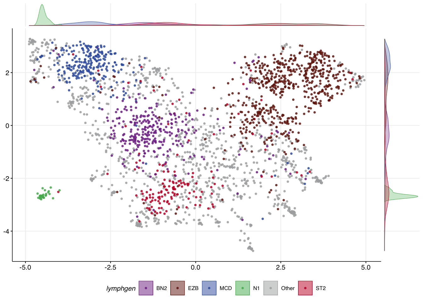
`make_and_annotate_umap`

mu_everything = make_and_annotate_umap(
  best_opt_model_matrix,
  dlbcl_meta_clean,
  core_features = list(
    ST2=c("SGK1","DUSP2","TET2","SOCS1"),
    N1="NOTCH1",
    EZB=c("EZH2","BCL2_SV"),
    MCD=c("MYD88HOTSPOT","CD79B","PIM1"),
    BN2=c("BCL6_SV","NOTCH2","SPEN","CD70")
  )
)

make_umap_scatterplot

make_umap_scatterplot(
  mu_everything$df,
  drop_other = F
)

DLBCLone_optimize_params

best_opt_model = DLBCLone_optimize_params(  
  mu_everything$features, 
  dlbcl_meta_clean,
  umap_out = mu_everything,
  truth_classes = c("MCD","EZB","BN2","N1","ST2","Other"),
  optimize_for_other = T,
  min_k=5,
  max_k=13
)

make_alluvial

DLBCLone with outgroup optimization (“wo”) w for weighted, o for optimized for other.

make_alluvial(best_opt_model,pred_column = "DLBCLone_wo",pred_name = "DLBCLone_wo")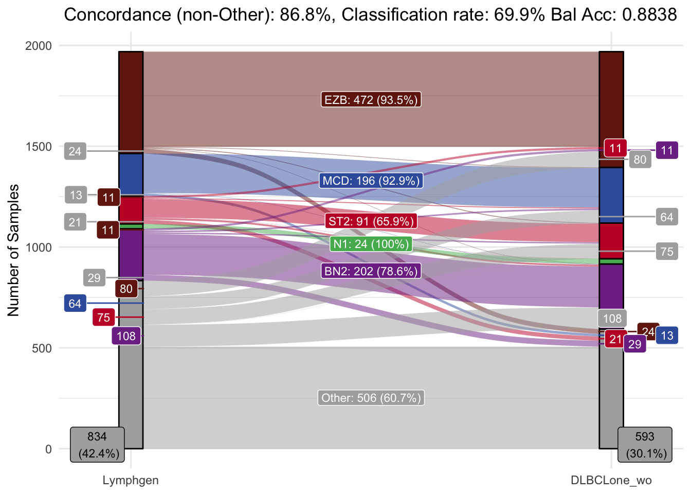

DLBCLone_predict

predicting one training sample

test_sample = "00-14595_tumorC"

pred_train <- DLBCLone_predict(
  mutation_status = best_opt_model_matrix[test_sample,],
  optimized_model = best_opt_model
)
knitr::kable(head(pred_train$prediction))

sample_id	predicted_label	confidence	other_score	neighbor_id	neighbor	distance	label	other_neighbor	vote_labels	weighted_votes	neighbors_other	neighborhood_otherness	other_weighted_votes	total_w	pred_w	V1	V2	.id	EZB_NN_count	MCD_NN_count	ST2_NN_count	N1_NN_count	BN2_NN_count	Other_NN_count	top_group	EZB_score	MCD_score	ST2_score	N1_score	BN2_score	Other_score	top_score_group	top_group_score	top_group_count	Other_count	by_vote	by_vote_opt	by_score	score_ratio	by_score_opt	DLBCLone_w	DLBCLone_wo
00-14595_tumorC	EZB	1	0	DLBCL11584T,CLC03456,DLBCL11428T,05-32762T,LY_RELY_116_tumorA,99-13280T,05-25439T,QC2-32T,SP193546,SP193976,14-20962T,FL1018T2,10-36955_tumorB	1112,351,995,85,1265,416,80,1322,1182,1164,247,89,172	0.203,0.223,0.231,0.259,0.265,0.293,0.297,0.306,0.321,0.34,0.345,0.349,0.352	EZB,EZB,EZB,EZB,EZB,EZB,EZB,EZB,EZB,EZB,EZB,EZB,EZB		EZB	46.055835675141	0	0	0	46.05584	46.05584	-3.826784	2.487499	1	13	0	0	0	0	0	EZB	46.05584	0	0	0	0	0	EZB	46.05584	13	0	13	EZB	EZB	Inf	EZB	EZB	EZB

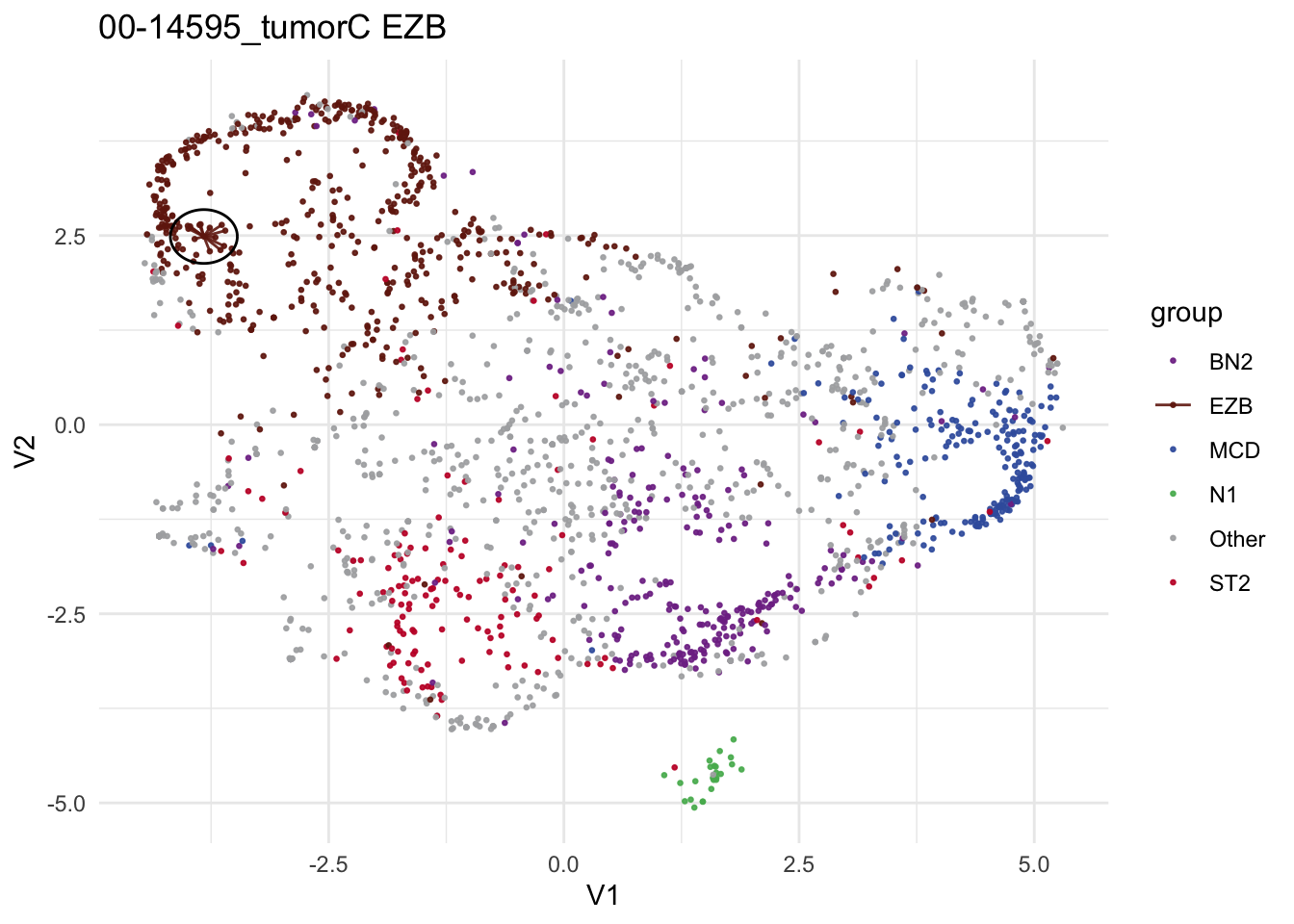
make_neighborhood_plot

make_neighborhood_plot(
  single_sample_prediction_output = pred_train,
  this_sample_id = "00-14595_tumorC",
  prediction_in_title = TRUE,
  add_circle = TRUE,
  label_column = "DLBCLone_wo"
)

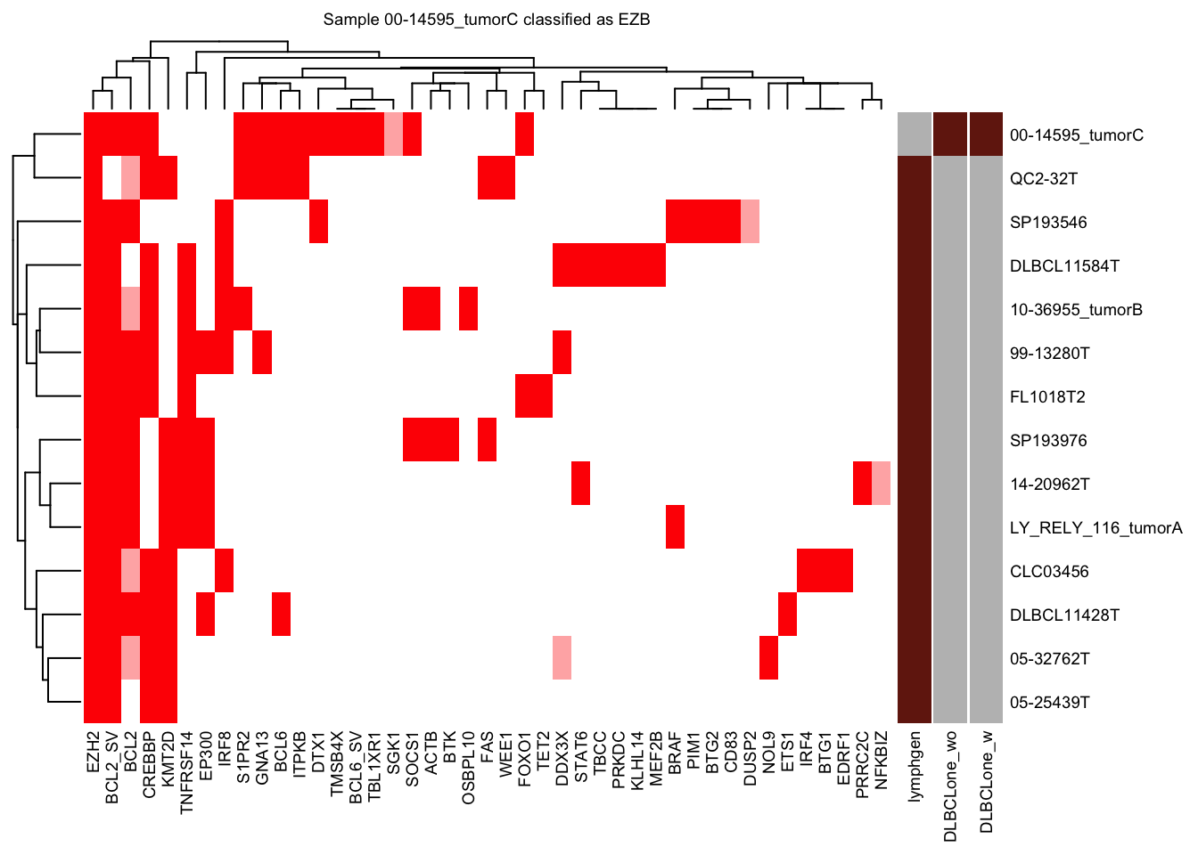
nearest_neighbor_heatmap

nearest_neighbor_heatmap(
  this_sample_id = "00-14595_tumorC",
  DLBCLone_model = pred_train,
  font_size = 7
)