library(GAMBLR.open)
library(GAMBLR.utils)
library(tidyverse)
library(GAMBLR.predict)

lymphgen_test = "extdata/lyseq_validation/LySeqST_only_unaugmented_vaf.lymphgen_calls.no_cnvs.with_sv.no_A53.tsv"
valid_metadata <- readr::read_tsv(
  system.file(lymphgen_test,package = "GAMBLR.predict")) %>%
  rename(
    sample_id = Sample.Name,
    lymphgen = Subtype.Prediction
  ) %>%
  mutate(
    BCL2.Translocation = if_else(BCL2.Translocation == "yes", "POS", BCL2.Translocation),
    BCL2.Translocation = if_else(BCL2.Translocation == "no", "NEG", BCL2.Translocation),
    BCL2.Translocation = if_else(BCL2.Translocation == "Not Available", "NA", BCL2.Translocation),
    BCL6.Translocation = if_else(BCL6.Translocation == "yes", "POS", BCL6.Translocation),
    BCL6.Translocation = if_else(BCL6.Translocation == "no", "NEG", BCL6.Translocation),
    BCL6.Translocation = if_else(BCL6.Translocation == "Not Available", "NA", BCL6.Translocation)
  )
maf_test = "extdata/lyseq_validation/LySeqST_merged_unaugmented_vaf.maf"
valid_maf_vaf_dir <- readr::read_tsv(system.file(maf_test,package = "GAMBLR.predict")) %>%
  mutate(
    sample_id = Tumor_Sample_Barcode
  )
#convert to S3 object for compatability
valid_maf_vaf <- create_maf_data(
    maf_df = valid_maf_vaf_dir,
    genome_build = "grch37"
  ) %>%
mutate(Chromosome = as.character(Chromosome))Applying a DLBCLone model to new data
Preamble
This guide will demonstrate the steps for training a custom DLBCLone model and applying it to classify new samples.
Preparing your test data
To use a trained DLBCLone model on your data, you need (at a minimum) either a MAF file or a mutation status matrix for the genes (features) that were used to generate the model. Here, you will learn how to generate a mutation status matrix using one of our published cohorts, which was sequenced with the LySeqST panel. If you have translocation status for BCL2, BCL6 etc and want to include that in the model, you will also need a second table that includes the translocation status for each sample. We generally refer to this as the metadata table. Together, your MAF and metadata files will be used to assemble the feature matrix that will be used for UMAP and KNN approximation on your samples.
SV status
For this example, we will extract the BCL2 and BCL6 status directly from the output of LymphGen. We will also use the LymphGen classification to evaluate our accuracy. Importantly, you do not need a LymphGen result from your test data but it can be useful to sanity check your UMAP and your model performance. The MAF and metadata for these samples (in the form of a LymphGen output) are both bundled with this package. The code below loads these files and restructures a few columns to make them compatible with downstream functions.
Synonymous mutations
If the model you’re using used base-3 encoding (0,1,2), that means synonymous mutations are considered for some genes. You will have to know up-front (or find out) which genes this applies to, so you can encode your data consistently. If your MAF file doesn’t contain any synonyous mutations, be sure to use a model that was trained only on coding mutations.
metadata
| sample_id | Copy.Number | BCL2.Translocation | BCL6.Translocation | Model.Used | Confidence.BN2 | Confidence.EZB | Confidence.MCD | Confidence.N1 | Confidence.ST2 | BN2.Feature.Count | EZB.Feature.Count | MCD.Feature.Count | N1.Feature.Count | ST2.Feature.Count | BN2.Features | EZB.Features | MCD.Features | N1.Features | ST2.Features | lymphgen |
|---|---|---|---|---|---|---|---|---|---|---|---|---|---|---|---|---|---|---|---|---|
| 00-14595_tumorA | Not Available | POS | POS | NOCGH | 0.79 | 0.99 | 0.00 | 0.07 | 0.03 | 3 | 3 | 1 | 0 | 2 | BCL6FusionCatcherORInHouse_FUSION,DTX1_MUTATION,BTG2_SubSyn | BCL2TransFISHMUTFusion_CompUp,EZH2_SubMUTATION,SOCS1_MUTATION | BTG2_SubSyn | NA | SOCS1_MUTATION,ITPKB_MUTATION | EZB |
| 00-14595_tumorB | Not Available | POS | POS | NOCGH | 0.79 | 0.99 | 0.00 | 0.07 | 0.68 | 3 | 3 | 3 | 0 | 3 | BCL6FusionCatcherORInHouse_FUSION,DTX1_MUTATION,BTG2_SubSyn | BCL2TransFISHMUTFusion_CompUp,EZH2_SubMUTATION,SOCS1_MUTATION | TBL1XR1_MUTATION,PIM2_SubSyn,BTG2_SubSyn | NA | SGK1_TRUNC,SOCS1_MUTATION,ITPKB_MUTATION | EZB |
| 00-14595_tumorC | Not Available | POS | POS | NOCGH | 0.79 | 0.99 | 0.00 | 0.07 | 0.68 | 3 | 4 | 3 | 0 | 3 | BCL6FusionCatcherORInHouse_FUSION,DTX1_MUTATION,BTG2_SubSyn | BCL2TransFISHMUTFusion_CompUp,EZH2_SubMUTATION,KMT2D_TRUNC,SOCS1_MUTATION | TBL1XR1_MUTATION,PIM2_SubSyn,BTG2_SubSyn | NA | SGK1_TRUNC,SOCS1_MUTATION,ITPKB_MUTATION | EZB |
| 00-14595_tumorD | Not Available | POS | NEG | NOCGH | 0.17 | 0.98 | 0.00 | 0.07 | 0.00 | 2 | 2 | 2 | 0 | 0 | DTX1_MUTATION,BTG2_SubSyn | BCL2TransFISHMUTFusion_CompUp,EZH2_SubMUTATION | PIM2_SubSyn,BTG2_SubSyn | NA | NA | EZB |
| 00-15201_tumorA | Not Available | NEG | NEG | NOCGH | 0.07 | 0.05 | 0.05 | 0.07 | 0.15 | 1 | 1 | 3 | 0 | 3 | TNFAIP3_TRUNC | KMT2D_TRUNC | PIM1_Synon,BTG1_SubSyn,HLA-A_MUTATION | NA | CD83_Synon,DUSP2_MUTATION,WEE1_Synon | Other |
| 00-15201_tumorB | Not Available | NEG | NEG | NOCGH | 0.18 | 0.11 | 0.01 | 0.99 | 0.00 | 2 | 1 | 3 | 1 | 0 | TNFAIP3_TRUNC,KLF2_Synon | EP300_MUTATION | HLA-B_MUTATION,PIM2_SubSyn,HLA-A_MUTATION | NOTCH1_MUTATION | NA | N1 |
lyseq features
The LySeqST sequencing panel includes the following genes. In order to train a classifier compatible with this panel, we need to subset the training data to ensure only these genes are included in training.
lyseq_genes <- c(
  "TNFRSF14", "SPEN", "ID3", "ARID1A", "RRAGC",
  "BCL10", "CD58", "NOTCH2", "FCGR2B", "FCRLA",
  "FAS", "CCND1", "BIRC3", "ATM", "KMT2D",
  "STAT6", "BTG1", "FOXO1", "B2M", "MAP2K1",
  "IDH2", "CHD2", "CREBBP", "SOCS1", "IL4R",
  "PLCG2", "TP53", "STAT5B", "STAT3", "CD79B",
  "GNA13", "BCL2", "TCF3", "S1PR2", "JAK3",
  "MEF2B", "DNMT3A", "XPO1", "CXCR4", "SF3B1",
  "PTPN1", "XBP1", "EP300", "MYD88", "SETD2",
  "RHOA", "NFKBIZ", "TBL1XR1", "KLHL6", "TET2",
  "PIM1", "CCND3", "TMEM30A", "PRDM1", "SGK1",
  "TNFAIP3", "CARD11", "POT1", "BRAF", "EZH2",
  "UBR5", "MYC", "NOTCH1", "TRAF2", "P2RY8",
  "BTK", "TP73", "NOL9", "SEMA4A", "PRRC2C",
  "BTG2", "ITPKB", "SEC24C", "EDRF1", "WEE1",
  "MPEG1", "ETS1", "DTX1", "SETD1B", "NFKBIA",
  "ZFP36L1", "CIITA", "MBTPS1", "IRF8", "ACTG1",
  "KLHL14", "MED16", "CD70", "JUNB", "KLF2",
  "CD79A", "DYSF", "DUSP2", "BCL2L1", "PRDM15",
  "RFTN1", "OSBPL10", "EIF4A2", "BCL6", "IRF4",
  "FOXC1", "CD83",
  "HLA-A", "HLA-B", "PRRC2A", "TBCC", "INTS1",
  "ACTB", "PIK3CG", "PRKDC", "TOX", "CDKN2A",
  "GRHPR", "DDX3X", "PIM2", "UBE2A", "ETV6",
  "MS4A1", "CD19", "HNRNPD", "NFKBIE", "TMSB4X"
)
Making a compatible feature matrix
You create a mutation feature matrix with assemble_genetic_features. This can include mutation status and structural variant status for BCL2, BCL6, and MYC. By default, synonymous mutations will be encoded as 1 and SV and coding mutations will be encoded as 2. The genes for which synonymous mutations are considered are specified separately. The genes we commonly use are shown in the example below.
ashm_genes = c("ACTB","ACTG1","BCL2","BCL6","BIRC3",
     "BTG1","BTG2","CD83","CIITA","CXCR4","DDX3X",
     "DTX1","DUSP2","ETS1","ETV6","GRHPR","ID3",
     "IL4R","IRF4","IRF8","ITPKB","KLF2","KLHL6",
     "MEF2B","MS4A1","MYC","NFKBIZ","OSBPL10","PIM1",
     "PIM2","PTPN1","RFTN1","S1PR2","SGK1","SOCS1",
     "TMSB4X","WEE1","XBP1","ZFP36L1")

lyseq_valid = assemble_genetic_features(
  these_samples_metadata = valid_metadata,
  sv_from_metadata = c(BCL2 = 'BCL2.Translocation', BCL6 = 'BCL6.Translocation'),
  genes=lyseq_genes,
  maf_with_synon = valid_maf_vaf,
  hotspot_genes = "MYD88",
  synon_genes=ashm_genes
)
Load the training data
all_full_status_train <- readr::read_tsv(system.file("extdata/all_full_status.tsv",package = "GAMBLR.predict")) %>%
  tibble::column_to_rownames("sample_id")

dlbcl_meta <- readr::read_tsv(system.file("extdata/dlbcl_meta_with_dlbclass.tsv",package = "GAMBLR.predict"))

dlbcl_meta_clean <- filter(dlbcl_meta,
                          lymphgen %in% c("MCD","EZB","BN2","N1","ST2","Other"))
Before training, the mutation matrix from the bundled training data must be subset to exclude any features that are not part of your panel.
Create training data UMAP
Visualize UMAP
Visually confirm the separation of the training samples based on their LymphGen class labels.
make_umap_scatterplot(mu_lyseq_train$df)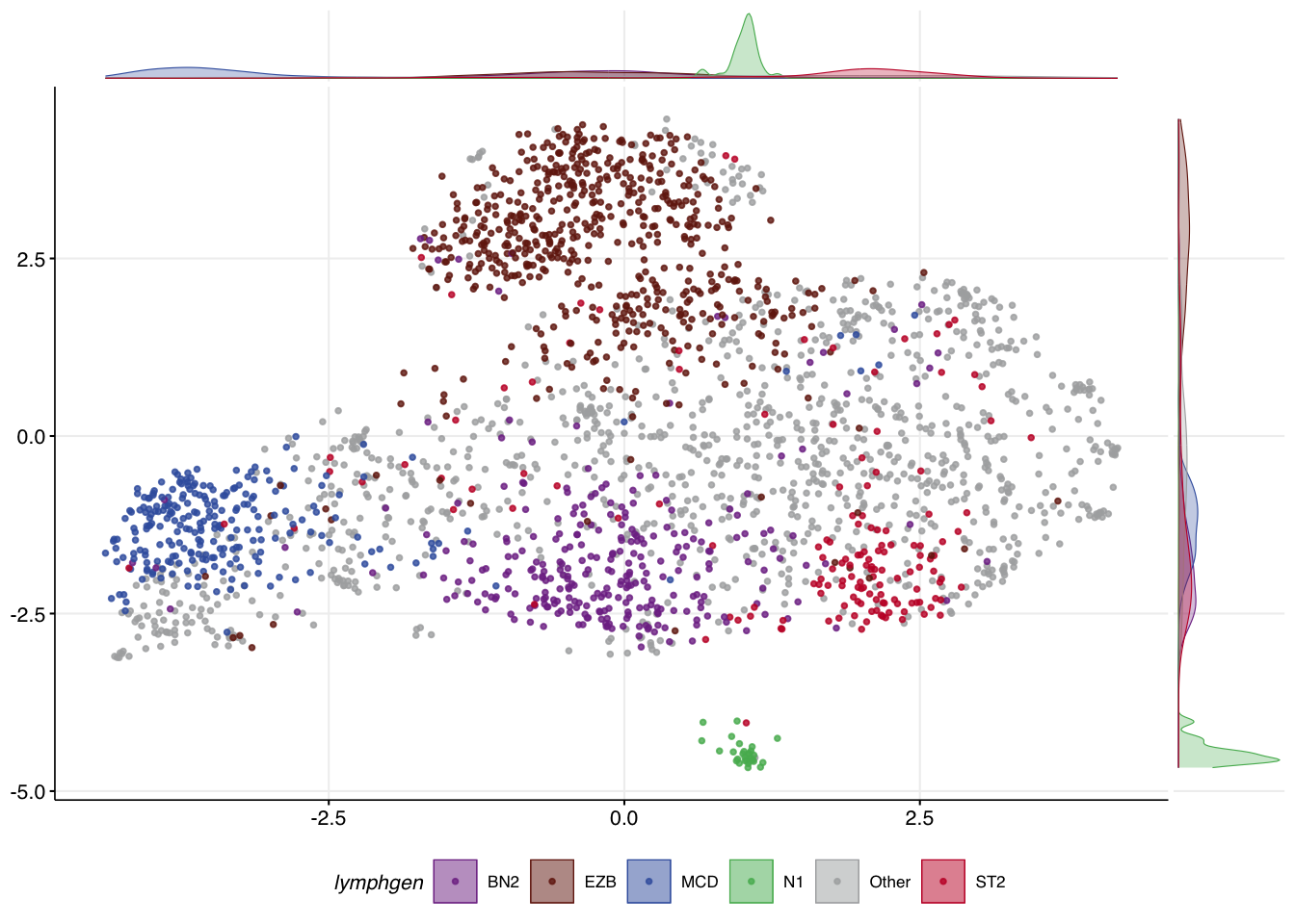
Train the model
Train and optimize our model using the training data with our custom feature set.
lyseq_features_optimized = DLBCLone_optimize_params(
  mu_lyseq_train$features,
  dlbcl_meta_clean,
  umap_out = mu_lyseq_train,
  truth_classes = c("MCD","EZB","BN2","N1","ST2","Other"),
  min_k=11,
  max_k=21
)

lyseq_features_optimized <- DLBCLone_activate( # Activates optimized model setting the UMAP projection
  lyseq_features_optimized,
  force = TRUE
)
lyseq_features_optimized <- DLBCLone_activate( # Activates optimized model setting the UMAP projection
  lyseq_features_optimized,
  force = TRUE
)
transforming each data point individually using the provided UMAP model. This will take some time.donemodel given to functionTraining accuracy
Check the classification accuracy of the optimized classifier (DLBCLone_wo) on the training data set.
make_alluvial(lyseq_features_optimized,
  pred_column="DLBCLone_wo")
Warning: Duplicated aesthetics after name standardisation: fillWarning in to_lodes_form(data = data, axes = axis_ind, discern =
params$discern): Some strata appear at multiple axes.
Warning in to_lodes_form(data = data, axes = axis_ind, discern =
params$discern): Some strata appear at multiple axes.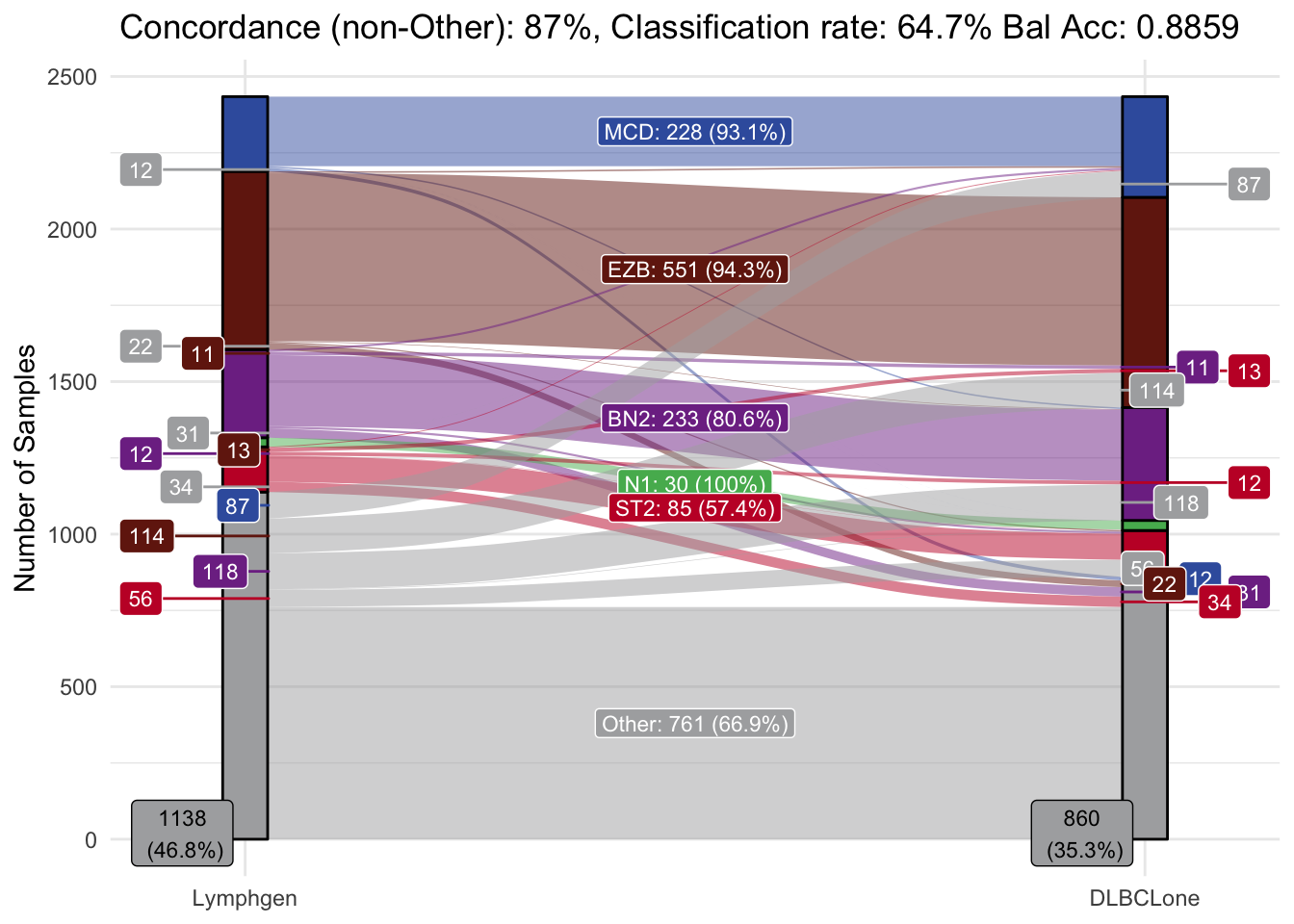
Sanity check feature incidence in the test data
pred_check <- DLBCLone_predict(
  mutation_status = lyseq_valid,
  optimized_model = lyseq_features_optimized,
  check_frequencies = TRUE
)
pred_check$plot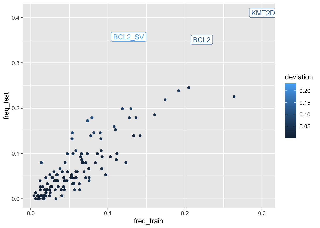
Apply the model to the test data
pred_valid_lyseq_all <- DLBCLone_predict(
  mutation_status = lyseq_valid,
  optimized_model = lyseq_features_optimized
)

knitr::kable(head(pred_valid_lyseq_all$prediction))| sample_id | predicted_label | confidence | other_score | neighbor_id | neighbor | distance | label | other_neighbor | vote_labels | weighted_votes | neighbors_other | neighborhood_otherness | other_weighted_votes | total_w | pred_w | V1 | V2 | .id | MCD_NN_count | EZB_NN_count | BN2_NN_count | N1_NN_count | ST2_NN_count | Other_NN_count | top_group | MCD_score | EZB_score | BN2_score | N1_score | ST2_score | Other_score | top_score_group | top_group_score | top_group_count | Other_count | by_vote | by_vote_opt | by_score | score_ratio | by_score_opt | DLBCLone_w | DLBCLone_wo |
|---|---|---|---|---|---|---|---|---|---|---|---|---|---|---|---|---|---|---|---|---|---|---|---|---|---|---|---|---|---|---|---|---|---|---|---|---|---|---|---|---|---|---|
| 00-14595_tumorA | EZB | 1.0000000 | 0.0000000 | 00-14595_tumorC,17-33848_tumorB,06-30025T,DLBCL11428T,09-41114T,03-11110T,06-30145T,SP116620,DLBCL-MC_F349_BJJ-Tumor,16-13732T,DLBCL11572T,CAR_154_PreCART,SU-DHL-4,05-25439T,DLBCL11656T,08-13706T,CAR_178_PreCART,05-25674T,06-18449_tumorB | 1,354,121,1106,172,47,122,1331,626,321,1218,508,2425,88,1240,140,515,89,109 | 0.128,0.142,0.145,0.149,0.152,0.156,0.195,0.205,0.212,0.223,0.227,0.244,0.251,0.251,0.251,0.26,0.271,0.274,0.288 | EZB,EZB,EZB,EZB,EZB,EZB,EZB,EZB,EZB,EZB,EZB,EZB,EZB,EZB,EZB,EZB,EZB,EZB,EZB | EZB | 95.7664551143418 | 0 | 0.0000000 | 0.000000 | 95.76646 | 95.76646 | -0.8899906 | 4.3290272 | 1 | 0 | 19 | 0 | 0 | 0 | 0 | EZB | 0.000000 | 95.76646 | 0.00000 | 0.00000 | 0.000000 | 0.000000 | EZB | 95.76646 | 19 | 0 | 19 | EZB | EZB | Inf | EZB | EZB | EZB | |
| 00-14595_tumorB | EZB | 1.0000000 | 0.0000000 | 09-41114T,03-11110T,00-14595_tumorC,17-33848_tumorB,DLBCL11428T,DLBCL-MC_F349_BJJ-Tumor,06-30025T,DLBCL11572T,SU-DHL-4,08-13706T,05-25439T,CAR_178_PreCART,CAR_154_PreCART,DLBCL11656T,SP116620,06-30145T,CAR_177_PreCART,06-18449_tumorB,DLBCL11567T | 172,47,1,354,1106,626,121,1218,2425,140,88,515,508,1240,1331,122,514,109,1213 | 0.113,0.115,0.13,0.141,0.158,0.163,0.181,0.188,0.194,0.207,0.21,0.215,0.219,0.229,0.229,0.247,0.259,0.26,0.263 | EZB,EZB,EZB,EZB,EZB,EZB,EZB,EZB,EZB,EZB,EZB,EZB,EZB,EZB,EZB,EZB,EZB,EZB,EZB | EZB | 103.880530854753 | 0 | 0.0000000 | 0.000000 | 103.88053 | 103.88053 | -0.8807368 | 4.2731309 | 2 | 0 | 19 | 0 | 0 | 0 | 0 | EZB | 0.000000 | 103.88053 | 0.00000 | 0.00000 | 0.000000 | 0.000000 | EZB | 103.88053 | 19 | 0 | 19 | EZB | EZB | Inf | EZB | EZB | EZB | |
| 00-14595_tumorC | EZB | 1.0000000 | 0.0000000 | 08-13706T,CAR_177_PreCART,CLC03454,SU-DHL-4,DLBCL11567T,DLBCL11572T,DLBCL-MC_F349_BJJ-Tumor,SP116659,CLC00259,CAR_154_PreCART,06-18449_tumorB,DLBCL-MC_F300_TBF-Tumor,DLBCL10459T,CAR_178_PreCART,02-13135T,05-32762T,FL1002T2,09-41114T,DLBCL10465T | 139,513,356,2424,1212,1217,625,1338,188,507,108,621,831,514,28,93,10,171,836 | 0.132,0.159,0.161,0.163,0.165,0.167,0.172,0.18,0.181,0.192,0.193,0.197,0.197,0.197,0.228,0.229,0.231,0.233,0.235 | EZB,EZB,EZB,EZB,EZB,EZB,EZB,EZB,EZB,EZB,EZB,EZB,EZB,EZB,EZB,EZB,EZB,EZB,EZB | EZB | 102.42382208477 | 0 | 0.0000000 | 0.000000 | 102.42382 | 102.42382 | -0.9343416 | 4.1505504 | 3 | 0 | 19 | 0 | 0 | 0 | 0 | EZB | 0.000000 | 102.42382 | 0.00000 | 0.00000 | 0.000000 | 0.000000 | EZB | 102.42382 | 19 | 0 | 19 | EZB | EZB | Inf | EZB | EZB | EZB | |
| 00-14595_tumorD | EZB | 1.0000000 | 0.0409382 | 190806-PL01-PL02,DLBCL11666T,DLBCL-MC_F358_WDS-Tumor,DLBCL11573T,05-25674T,10-15025T,Aph_13_PreCART,DLBCL11558T,FL1010T2,SU-DHL-6,SP116620,06-15922T,SP194216,CAR_276_PreCART,DLBCL11575T,SP193957,171290-PL01,170867-PL02,15-11280_CLC02281 | 450,1249,627,1219,89,177,469,1206,449,2427,1331,105,1301,526,1220,1307,461,460,285 | 0.118,0.126,0.154,0.157,0.159,0.166,0.173,0.18,0.202,0.204,0.207,0.21,0.21,0.234,0.236,0.252,0.253,0.253,0.255 | EZB,EZB,EZB,EZB,EZB,EZB,EZB,EZB,EZB,EZB,EZB,EZB,EZB,EZB,EZB,EZB,EZB,EZB,EZB | FL1003T2 | EZB | 101.424039965503 | 1 | 0.0526316 | 4.152118 | 101.42404 | 101.42404 | -0.6999627 | 4.4204650 | 4 | 0 | 19 | 0 | 0 | 0 | 0 | EZB | 0.000000 | 101.42404 | 0.00000 | 0.00000 | 0.000000 | 4.152118 | EZB | 101.42404 | 19 | 1 | 19 | EZB | EZB | 24.4270604 | EZB | EZB | EZB |
| 00-15201_tumorA | BN2 | 0.4536479 | 8.6321139 | Reddy_3551T,Reddy_2620T,Reddy_2789T,Reddy_3904T,DLBCL11518T,SP116690,DLBCL-c_D_1158-Tumor,Reddy_2650T,1011-2020_FFPE,DLBCL-RICOVER_978-Tumor,Reddy_2603T,Reddy_2534T,Reddy_3616T,QC2-30T,DLBCL10856T,DLBCL10919T,Reddy_705T,Reddy_3849T,H041_T_WGS | 2076,1768,1862,2315,1184,1343,813,1788,218,761,1756,1714,2112,1503,941,999,2411,2279,600 | 0.189,0.233,0.484,0.491,0.569,0.575,0.624,0.679,0.681,0.683,0.722,0.739,0.821,0.857,0.859,0.865,0.888,0.91,0.952 | BN2,BN2,ST2,ST2,BN2,ST2,ST2,EZB,EZB,BN2,EZB,BN2,BN2,EZB,EZB,EZB,EZB,EZB,MCD | 1102503091T,Reddy_3739T,Reddy_2147T,1102503011T,Reddy_3865T,DFCIDL008-Tumor,DLBCL10977T,1011-2018_FFPE,Reddy_3843T,Reddy_3819T,1011-2018_plasma,Reddy_2634T,DLBCL10933T,DLBCL-c_D_1120-Tumor,00-22011_tumorB,DLBCL11002T,DLBCL11595T,Reddy_2206T,1001-2030_FFPE,Reddy_3845T,1102503013T,Reddy_3733T,DLBCL10955T,OZM073-017_Diagnosis,Reddy_3988T,Reddy_3914T,Reddy_3519T,Reddy_3487T,Reddy_2996T,Reddy_2138T,03-10440_tumorB,03-10440_tumorA,DLBCL11468T,DLBCL-RICOVER_314-Tumor,Reddy_3580T,DLBCL11255T,DLBCL10455T,DLBCL10943T,Reddy_2463T,SP116627,Reddy_3431T,Reddy_2253T,Reddy_702T,Reddy_2123T,Reddy_3943T,Reddy_3556T,Reddy_3412T,Reddy_2714T,Reddy_2479T,Reddy_2719T,Reddy_3981T,02-15630_tumorB,Reddy_3978T,86-30788_tumorA,Reddy_813T,Reddy_2157T,Reddy_2889T,Seq_1_PreCART,94-15772_tumorA,Reddy_2928T,Reddy_2680T,QC2-5T,Reddy_2194T,DLBCL10499T,98-22532T,DLBCL10908T,DLBCL-c_D_1152-Tumor,Reddy_3470T,Reddy_3946T,94-15772_tumorB,DLBCL11180T,DLBCL11681T,Reddy_3654T,Reddy_2688T,1001-2030_plasma | BN2,EZB,MCD,ST2 | 15.3910313542603,10.0403628209901,1.05047600249142,7.44539197428758 | 75 | 3.9473684 | 132.857136 | 33.92726 | 15.39103 | -1.2391076 | 0.3538165 | 5 | 1 | 8 | 6 | 0 | 4 | 0 | EZB | 1.050476 | 10.04036 | 15.39103 | 0.00000 | 7.445392 | 132.857136 | BN2 | 15.39103 | 8 | 75 | 8 | Other | BN2 | 0.1158465 | Other | BN2 | Other |
| 00-15201_tumorB | N1 | 0.9709068 | 0.0466497 | DLBCL10973T,DLBCL11648T,10-39294_tumorA,DLBCL10520T,DLBCL11005T,14-33798_tumorB,DLBCL11503T,DLBCL11513T,10-39294_tumorB,DLBCL10844T,CLC00246,DLBCL-MAYO_DLBCL_234-Tumor,1102502995T,Reddy_3982T,DLBCL10915T,c_D_1050_T,DLBCL10952T,Reddy_3997T,DLBCL11439T | 1048,1235,186,885,1078,276,1172,1180,187,929,315,1442,1418,2384,995,1433,1028,2399,1115 | 0.173,0.183,0.224,0.264,0.284,0.288,0.289,0.293,0.389,0.412,0.478,0.486,0.5,0.528,0.529,0.542,0.571,0.613,0.623 | N1,N1,N1,N1,N1,N1,N1,N1,N1,N1,N1,N1,N1,N1,N1,N1,N1,N1,ST2 | 1102503029T | N1,ST2 | 53.5304488302436,1.6040359180294 | 1 | 0.0526316 | 2.497182 | 55.13448 | 53.53045 | 0.7030904 | -4.2771802 | 6 | 0 | 0 | 0 | 18 | 1 | 0 | N1 | 0.000000 | 0.00000 | 0.00000 | 53.53045 | 1.604036 | 2.497182 | N1 | 53.53045 | 18 | 1 | 18 | N1 | N1 | 21.4363427 | N1 | N1 | N1 |
Sanity check the UMAP
If the UMAP is working as it should be, you should see a similar level of separation of your test samples in UMAP space. Since we have LymphGen classifications for our test samples, we can check this. In order to visualize these, the metadata will need to be attached to the UMAP projection of the new samples. What you should hopefully see is roughly the same placement of your samples on this scatterplot relative to the training samples.
projected_with_meta = left_join(pred_valid_lyseq_all$projection,
select(valid_metadata,sample_id,lymphgen))
Joining with `by = join_by(sample_id)`
head(projected_with_meta) sample_id V1 V2 lymphgen
1 00-14595_tumorA -0.8899906 4.3290272 EZB
2 00-14595_tumorB -0.8807368 4.2731309 EZB
3 00-14595_tumorC -0.9343416 4.1505504 EZB
4 00-14595_tumorD -0.6999627 4.4204650 EZB
5 00-15201_tumorA -1.2391076 0.3538165 Other
6 00-15201_tumorB 0.7030904 -4.2771802 N1
unique(projected_with_meta$lymphgen) [1] "EZB" "Other" "N1" "BN2/N1" "BN2"
[6] "MCD" "ST2" "EZB/MCD/ST2" "EZB/ST2" "BN2/EZB"
[11] "BN2/MCD" "EZB/MCD"
make_umap_scatterplot(projected_with_meta)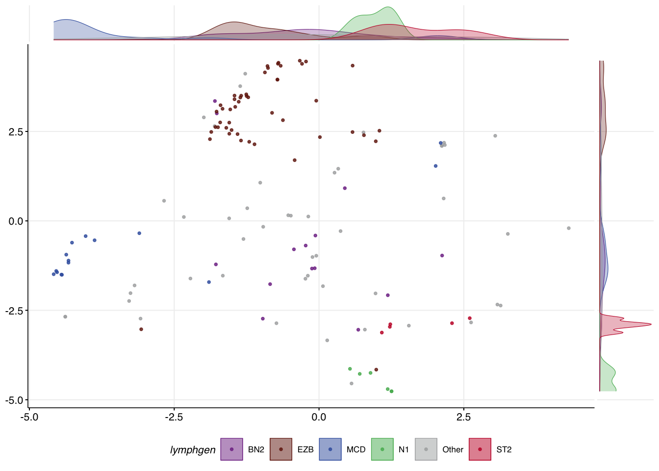
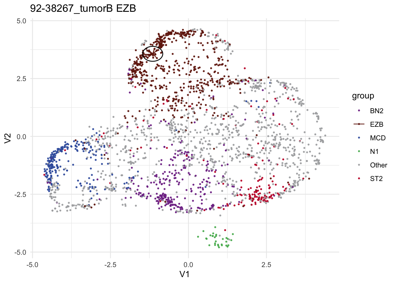
make_neighborhood_plot
test_sample = "92-38267_tumorB"

make_neighborhood_plot(
  single_sample_prediction_output = pred_valid_lyseq_all,
  this_sample_id = test_sample,
  prediction_in_title = TRUE,
  add_circle = TRUE,
  label_column = "DLBCLone_wo"
)
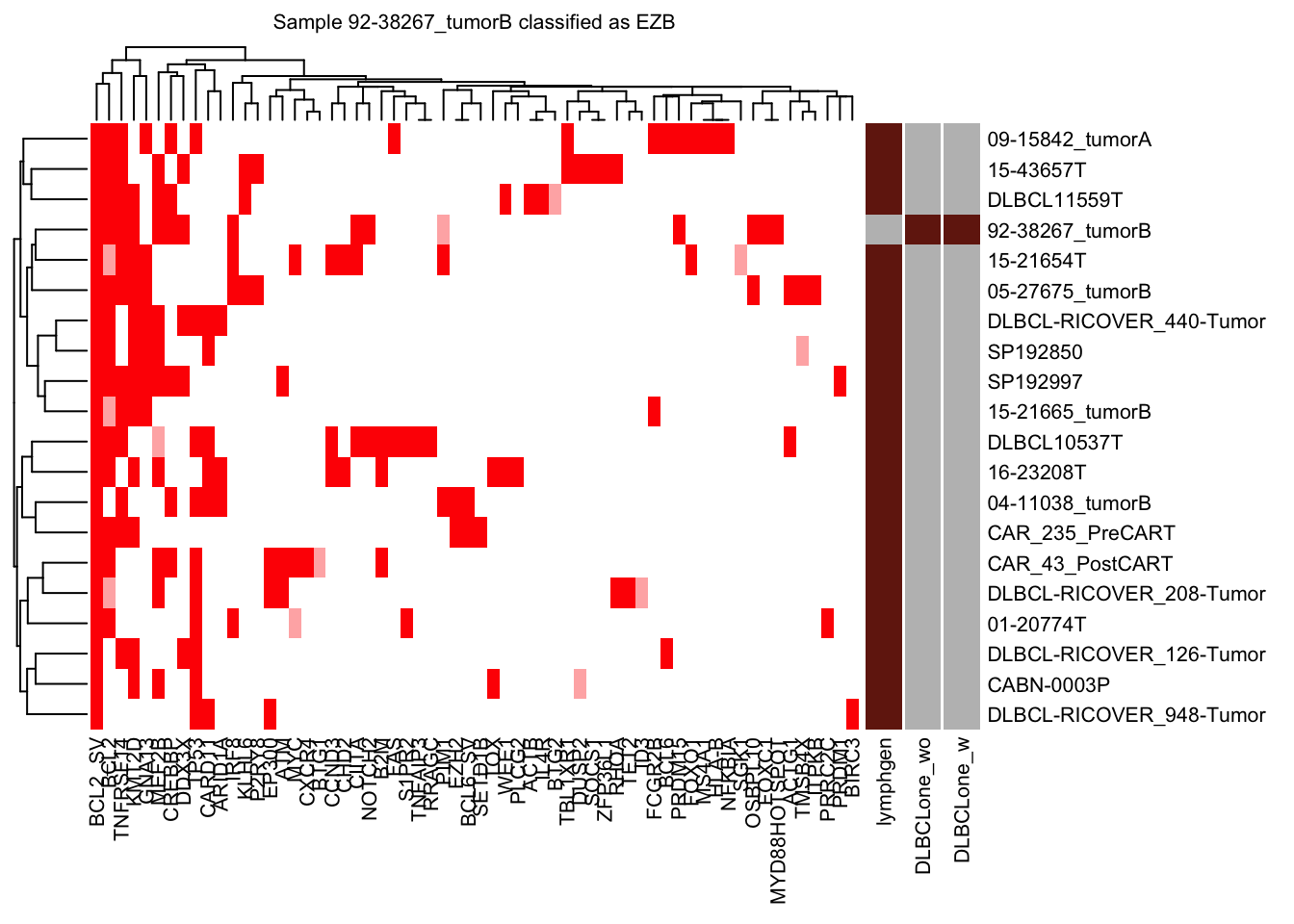
nearest_neighbor_heatmap
nearest_neighbor_heatmap(
  this_sample_id = test_sample,
  DLBCLone_model = pred_valid_lyseq_all,
  font_size = 8
)
Accuracy Assessment
Finally, lets assess the accuracy of the validation set by comparing dlbclone_predict predictions with the LymphGen results that were previously generated.
pred_vs_original = left_join(pred_valid_lyseq_all$prediction,valid_metadata)

#collapse composites into group-COMP
pred_vs_original = tidy_lymphgen(pred_vs_original,lymphgen_column_in = "lymphgen",lymphgen_column_out = "lymphgen_tidy")

#convert composites into their primary class
pred_vs_original = mutate(pred_vs_original,lymphgen_basic = gsub("-COMP","",lymphgen_tidy))

make_alluvial(list(predictions=pred_vs_original),
  pred_column = "DLBCLone_wo",
  group_order = c("MCD","BN2","ST2","EZB","N1","Other"),
  truth_column = "lymphgen_basic")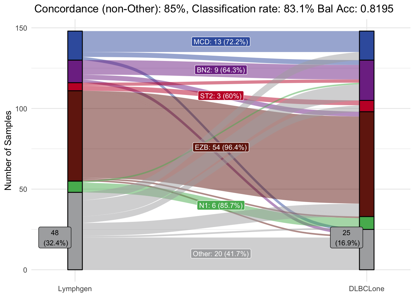
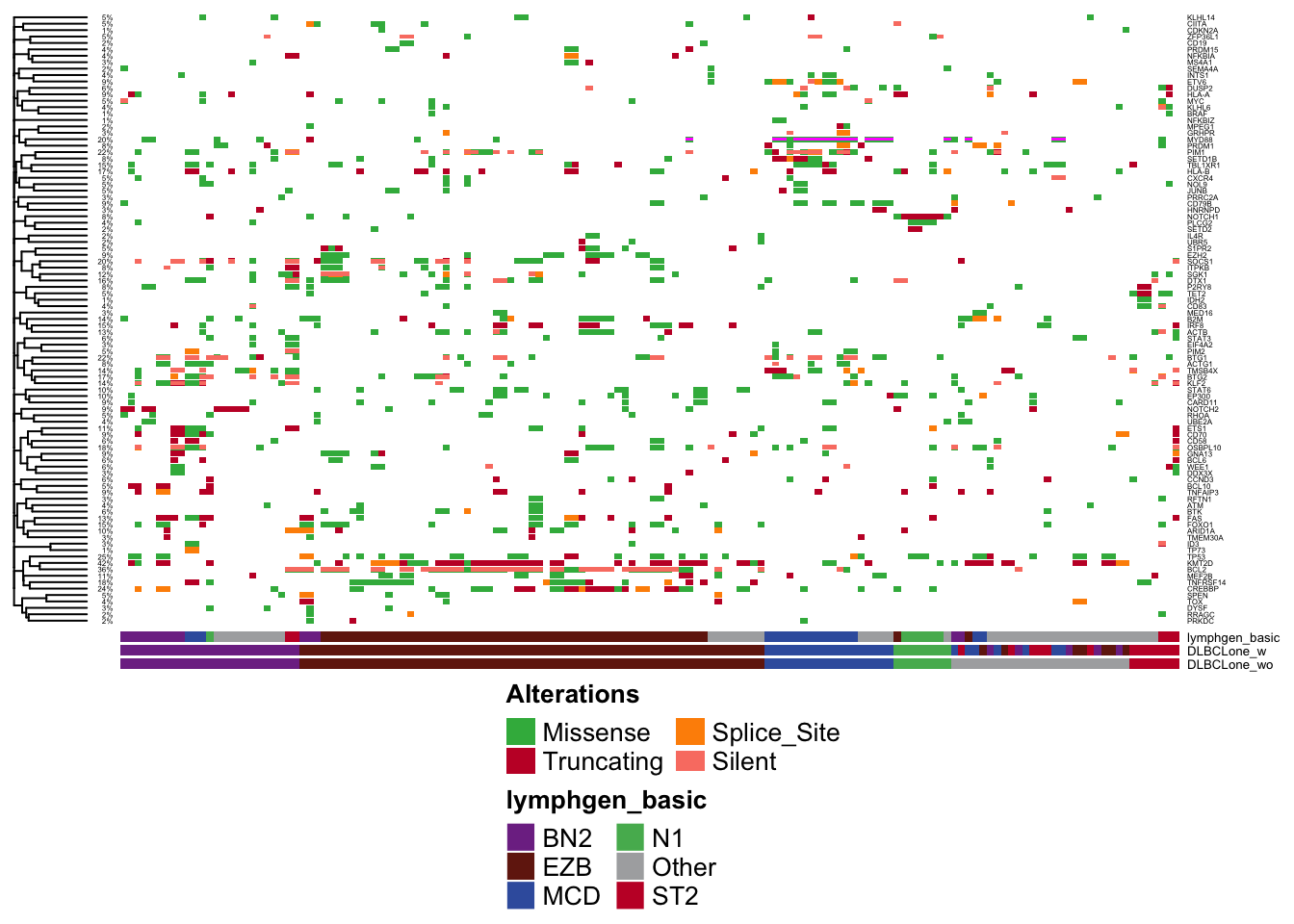
Oncoplot
Another way to visualize the results is via an Oncoplot (using GAMBLR.viz::prettyOncoplot).
library(GAMBLR.viz)
ashm_genes = intersect(ashm_genes,lyseq_genes)

silent_show = rep("Silent",length(ashm_genes))
names(silent_show)=ashm_genes
# add hotspot annotation
valid_maf_vaf$hot_spot = NA
valid_maf_vaf = mutate(valid_maf_vaf,hot_spot=ifelse(Hugo_Symbol=="MYD88" & HGVSp_Short=="p.L265P",TRUE,FALSE))
prettyOncoplot(these_samples_metadata = pred_vs_original,
  maf_df = valid_maf_vaf,
  metadataColumns = c("lymphgen_basic","DLBCLone_w","DLBCLone_wo"),
  minMutationPercent = 1,
  cluster_rows = T,
  highlightHotspots = T,
  genes = lyseq_genes,
  pctFontSize = 3,
  fontSizeGene = 3,
  hideSideBarplot = T,
  simplify_annotation = T,
  hide_annotations = c("DLBCLone_wo","DLBCLone_w"),
  include_noncoding = as.list(silent_show),
  sortByColumns = c("DLBCLone_wo","lymphgen_basic"))