Classifying samples with DLBCLone • GAMBLR.predict

Preamble

The most practical use for a DLBCLone model is to infer the class/subtype of samples based on the genetic features present. This is accomplished with the DLBCLone_predict function. This tutorial assumes you will start with a previously saved model, which you will restore from disk and re-activate as shown in the previous tutorial.

predicting the class of a single sample

In this demonstration, we’ll use our model to predict the class of one of our training samples. This is not the normal, or particularly sensible, application of DLBCLone but it’s a convenient way to demonstrate how DLBCLone_predict works. Since we’re using a sample that was in the training data, we can directly recycle the genetic feature matrix from the model via all_features_optimized$features. Because there are meta-features in that data frame, we also need to enable the drop_extra feature.

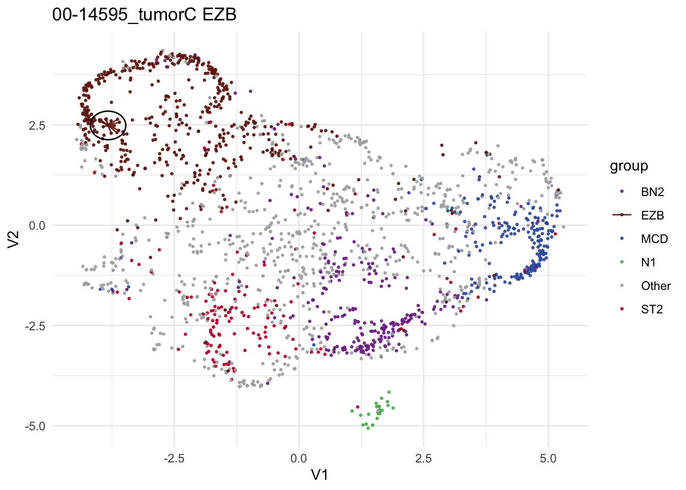
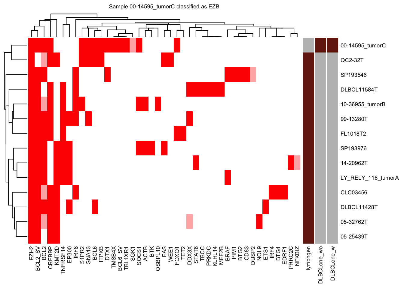
test_sample = "00-14595_tumorC"

pred_train <- DLBCLone_predict(
  mutation_status = all_features_optimized$features[test_sample,],
  optimized_model = all_features_optimized,
  drop_extra = TRUE
)

knitr::kable(head(pred_train$prediction))

sample_id	predicted_label	confidence	other_score	neighbor_id	neighbor	distance	label	other_neighbor	vote_labels	weighted_votes	neighbors_other	neighborhood_otherness	other_weighted_votes	total_w	pred_w	V1	V2	.id	EZB_NN_count	MCD_NN_count	ST2_NN_count	N1_NN_count	BN2_NN_count	Other_NN_count	top_group	EZB_score	MCD_score	ST2_score	N1_score	BN2_score	Other_score	top_score_group	top_group_score	top_group_count	Other_count	by_vote	by_vote_opt	by_score	score_ratio	by_score_opt	DLBCLone_w	DLBCLone_wo
00-14595_tumorC	EZB	1	0	DLBCL11584T,CLC03456,DLBCL11428T,05-32762T,LY_RELY_116_tumorA,99-13280T,05-25439T,QC2-32T,SP193546,SP193976,14-20962T,FL1018T2,10-36955_tumorB	1112,351,995,85,1265,416,80,1322,1182,1164,247,89,172	0.203,0.223,0.231,0.259,0.265,0.293,0.297,0.306,0.321,0.34,0.345,0.349,0.352	EZB,EZB,EZB,EZB,EZB,EZB,EZB,EZB,EZB,EZB,EZB,EZB,EZB		EZB	46.055835675141	0	0	0	46.05584	46.05584	-3.826784	2.487499	1	13	0	0	0	0	0	EZB	46.05584	0	0	0	0	0	EZB	46.05584	13	0	13	EZB	EZB	Inf	EZB	EZB	EZB

Visualizing a the neighborhood of a single classification

make_neighborhood_plot

Used for visualizing how and where neighbors are selected, a umap plot is produced showcasing the test sample of interest and its trained neighbors that helped determine its labeling.

single_sample_prediction_output output list from predict_single_sample_DLBCLone

training_predictions training predictions from DLBCLone_optimize_params (e.g. optimized_model$df)

this_sample_id Character the sample ID for which the neighborhood plot will be generated

prediction_in_title if TRUE: includes the predicted label in the plot title

add_circle Plot will include a circle surrounding the set of neighbors, helpful for identification

make_neighborhood_plot(
  single_sample_prediction_output = pred_train,
  this_sample_id = "00-14595_tumorC",
  prediction_in_title = TRUE,
  add_circle = TRUE,
  label_column = "DLBCLone_wo"
)

nearest_neighbor_heatmap

Generates a heatmap of feature values for the nearest neighbors of a specified sample, based on a DLBCLone model object. This visualization helps to inspect the feature profiles of samples most similar to the query sample.

this_sample_id the sample ID for which to plot the nearest neighbor heatmap

DLBCLone_model a DLBCLone model object, which can be the output of DLBCLone_optimize_params, DLBCLone_KNN, or DLBCLone_predict

truth_column the column name in the predictions data frame that contains the ground truth labels (default: “lymphgen”)

metadata_cols optional character vector of additional metadata columns to include in the heatmap annotations

clustering_dis the distance metric to use for clustering rows (default: “binary”)

font_size font size for heatmap text (default: 14)

nearest_neighbor_heatmap(
  this_sample_id = "00-14595_tumorC",
  DLBCLone_model = pred_train,
  font_size = 7
)