Utilities Tutorial
utilities_tutorial.RmdUtilities
In this vignette we are exploring functions that fall under the category, utilities. This is a collection of functions that can be used for a variety of applications, such as retrieving gene coordinates from regions (and the other way around), cleaning and sanitizing data, creating custom tracks for the UCSC Genome Browser, getting collated results, accessing the GAMBLR colour paletter, etc.
Genes, Regions and Statistical Computing
This section demonstrates how to return information related to genes and other specified genomic regions
Gene To Region
If you have a set of genes and you are interested in returning the genomic coordinates for these genes, it is recommended to call gene_to_region. This function takes four parameters; gene_symbol, a vector of on or more gene symbols in Hugo format. ensembl_id, a vector of one or more Ensembl IDs. genome_build, the desired projection for returned regions, acceptable values are hg38 and grch37. return_as, the format of returned regions, acceptable values are (1) region (a string formatted as chr:start-end), (2) bed and (3) df. Let’s have a look at a few different examples, using a few different parameter combinations.
#gene to region, for a single gene returned as "region"
myc_region = gene_to_region(gene_symbol = "MYC", genome_build = "grch37", return_as = "region")

#print region
myc_region
## [1] "8:128747680-128753674"
#gene to region, for multiple genes (MYC and BCL2) in a vector of characters, returned in bed format.
genes_bed = gene_to_region(ensembl_id = c("ENSG00000136997", "ENSG00000171791"), genome_build = "hg38", return_as = "bed")

#print regions
genes_bed
## chromosome start end hugo_symbol
## 1 chr18 63123345 63320128 BCL2
## 2 chr8 127735433 127742951 MYC
#gene to region, for multiple genes specified in an already subset list of gene names, return format is data frame
#subset FL genes
fl_genes = dplyr::filter(lymphoma_genes_lymphoma_genes_v0.0, FL == TRUE) %>% pull(Gene)

#get regions for Fl genes
fl_genes_df = gene_to_region(gene_symbol = fl_genes, genome_build = "grch37", return_as = "df")
Region To Gene
Similarly, we can also return genes that are residing within a specified region. For this purpose region_to_gene was developed. This function operates in a similar way as the previous described function. Three parameters are available for this function; region, regions to intersect genes with, this can be either a data frame with regions sorted in the following columns; chromosome, start, end. Or it can be a character vector in “region” format, i.e chromosome:start-end. gene_format, parameter for specifying the format of returned genes, default is “hugo”, other acceptable inputs are “ensembl”. genome_build, the desired projection for returned regions, acceptable values are hg38 and grch37. Here are a few examples showcasing how the different parameters can be used, as well as examples on how to make the most out of this function.
#simple example using a previously defined region (MYC)
genes_in_this_region = region_to_gene(region = myc_region, gene_format = "hugo", genome_build = "grch37")

#print genes
genes_in_this_region
## chromosome start end hugo_symbol region_start region_end
## 1 chr8 128747680 128753674 MYC 128747680 128753674
#wider example using larger region (q-arm, chromosome 1) and using another genome build (hg38) and gene format (ensembl)
chr1q_genes = region_to_gene(region = "chr1:143200000-248956422", gene_format = "ensembl", genome_build = "hg38")
Regions To Bins
This function was developed to split a contiguous genomic region on a chromosome into non-overlapping bins. This function takes four parameter; chr, start, end, and bin_size. In this example we are splitting the q-arm on chromosome 8 into bins of 20000 base pairs.
#regions to bin, bin chromosome 8 into 20000 bins
chr8q_bins = region_to_bins(chromosome = "8", start = 48100000, end = 146364022, bin_size = 20000)
Count SSM by Region
Sometimes it can be helpful to tally all mutations (SSM) in a region for a set number of samples. To do so, one can call count_ssm_by_region. This function takes genomic coordinates either specified in region format (chr:start-end) with the region parameter, or the chromosome, start and end can be specified individually with the chr, start, and end parameters. In this example we are first creating a metadata subset, only including samples with FL as the pathology. Next, we are defining a region for MYC with help from gene_to_region with he return format specified as “region”. The return is the sum of all SSMs overlapping with MYC for all FL samples.
#define a region.
my_region = gene_to_region(gene_symbol = "MYC", return_as = "region")

#subset metadata.
my_metadata = get_gambl_metadata() %>%
  dplyr::filter(pathology == "FL")

#count SSMs for the selected sample subset and defined region.
fl_ssm_counts_myc = count_ssm_by_region(region = my_region, these_samples_metadata = my_metadata)

#print number of SSMs in the defined region for the selected samples
print(fl_ssm_counts_myc)
## [1] 12Coding SSM Status
Another way to summarize SSM across samples for coding regions is with get_coding_ssm_status. This function takes a list of gene symbols and subsets the incoming MAF to specified genes. If no gene list is provided, the function will default to all lymphoma genes. The function can accept a wide range of incoming MAFs. For example, the user can call this function with these_samples_metadata (preferably a metadata table that has been subset to the sample IDs of interest). If this parameter is not called, the function will default to all samples available with get_gambl_metadata. The user can also provide a path to a MAF, or MAF-like file with maf_path, or an already loaded MAF can be used with the maf_data parameter. If both maf_path and maf_data is missing, the function will default to run get_coding_ssm. In this example, we are returning the mutation status for FL samples (using the already subset metadata table from the previous example) in respect to MYC.
#tabulate coding SSMs for FL samples.
coding_tabulated_df = get_coding_ssm_status(these_samples_metadata = my_metadata, review_hotspots = FALSE, include_hotspots = FALSE, gene_symbols = "MYC")
Calculate Proportion of Genome Altered by CNV
Interested to see the percentage of a genome altered by CNVs for specific sample, or sample subsets? For this purpose calcualte_pga was developed. This function takes into account the total length of sample’s CNV and relates it to the total genome length to return the proportion affected by CNV. The function can work with either individual or multi-sample seg files. The telomeres are always excluded from calculation, and centromeres/sex chromosomes can be optionally included or excluded.
#get CN segments for a specific sample.
sample_seg = get_sample_cn_segments(this_sample_id = "14-36022T") %>%
  dplyr::rename("sample" = "ID")

#calculate PGA for the same sample.
calculate_pga(this_seg = sample_seg)
## sample_id PGA
## 1 14-36022T 0.871Adjust Ploidy
The adjust_ploidy function returns a seg file with log.ratios adjusted to the overall sample ploidy. This function adjusts the ploidy of the sample using the percent of genome altered (PGA). The PGA is calculated internally, but can also be optionally provided as data frame if calculated from other sources. Only the samples above the threshold-provided PGA (pga_cutoff) will have ploidy adjusted. The function can work with either individual or multi-sample seg file.
#ajdust ploidy
adjust_ploidy(this_seg = sample_seg)
## # A tibble: 187 × 6
## sample chrom start end LOH_flag log.ratio
## <chr> <chr> <dbl> <dbl> <dbl> <dbl>
## 1 14-36022T 1 10001 762600 0 0
## 2 14-36022T 1 762601 121500000 0 0
## 3 14-36022T 1 142600000 248277662 0 0
## 4 14-36022T 1 248277663 248278622 0 0
## 5 14-36022T 1 248278623 249226346 0 -1
## 6 14-36022T 1 249226347 249250620 0 0
## 7 14-36022T 2 10001 11319 0 0
## 8 14-36022T 2 11320 90500000 0 0
## 9 14-36022T 2 96800000 186704965 0 0
## 10 14-36022T 2 186704966 186712276 0 0
## # ℹ 177 more rowsCompare CNVs For Multiple Samples
cnvKompare will compare CNV data between samples with multiple time points. It can also handle same-sample comparison between different CNV callers if the sample ID is specified in unique fashion. For groups with more than 2 samples, optionally pairwise comparisons can be performed. The comparison is made based on the internally calculated score, which reflects the percentage of each cytoband covered by CNV (rounded to the nearest 5%) and its absolute CN. Optionally, the heatmap of cnvKompare scores can be returned. In addition, the function will return all concordant and discordant cytobands. Finally, the time series plot of CNV log ratios will be returned for all lymphoma genes, with further functionality to subset it to a panel of genes of interest.
#get CNV comparison data.
kompare_out = cnvKompare(patient_id = "13-26835",
                         projection = "hg38",
                         show_x_labels = FALSE,
                         genes_of_interest = c("EZH2",
                                               "TP53",
                                               "MYC",
                                               "CREBBP",
                                               "GNA13"))
# concordance as percent
kompare_out$overall_concordance_pct
## [1] 12.12
#visualizations
kompare_out$Heatmap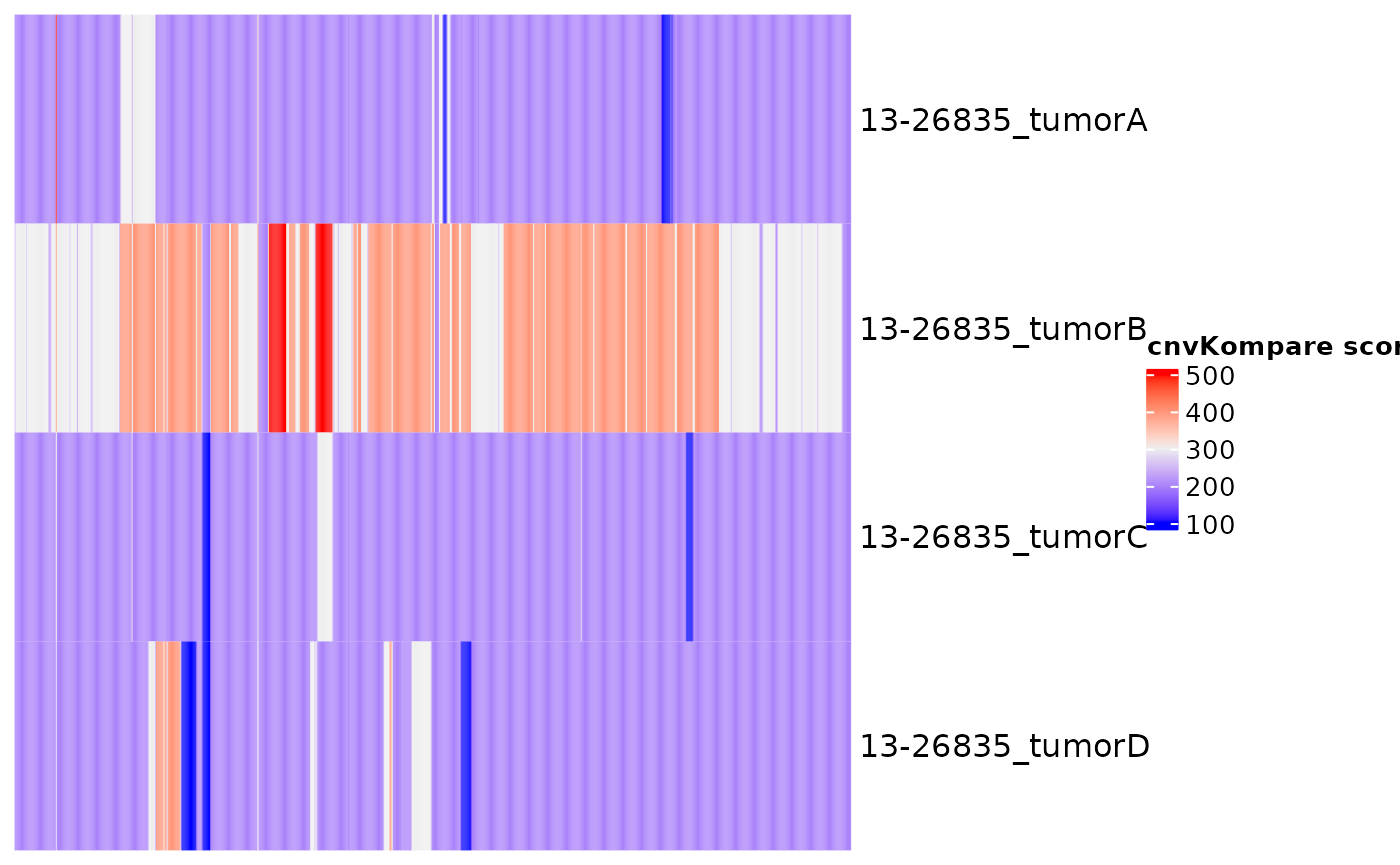
kompare_out$time_plot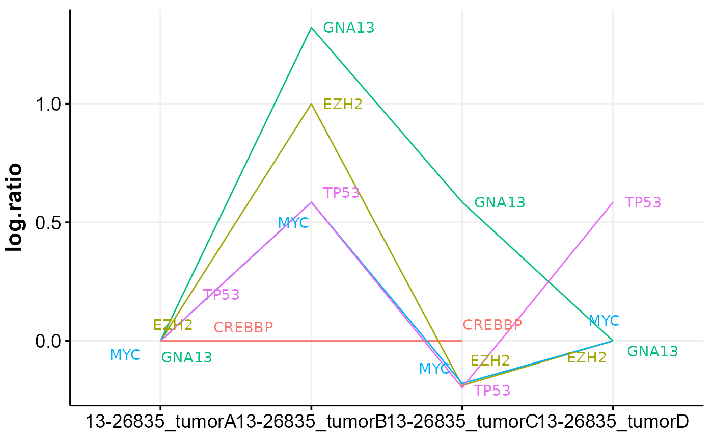
Genome to Exome
If you are interested to subset a maf to only features that would be available in Whole Genome Exome (WEX) data, genome_to_exome is available for this purpose. This function takes the following parameters; maf, the incoming maf object. Can be maf-like data frame or maftools maf object. Minimum columns that should be present are Chromosome, Start_Position, and End_Position. custom_bed, optional argument specifying a path to custom bed file for covered regions. Must be bed-like and contain chrom, start, and end position information in first 3 columns. Other columns are disregarded if provided. genome_build, string indicating genome build of the maf file. Default is grch37, but can accept modifications of both grch37- and hg38-based builds. padding, numeric value that will be used to pad probes in WEX data from both ends. Default is 100. After padding, overlapping features are squished together. let’s have a look at an example using this function.
#get all ssm in the MYC aSHM region
myc_ashm_maf = get_ssm_by_region(region = "8:128748352-128749427")

#get mutations with 100 bp padding (default)
wex = genome_to_exome(maf = myc_ashm_maf)
Miscellaneous
Collate Results
Collate Results is used to retrieve a vast collection of sample-level results and summary data, generated by individual GAMBL pipelines. All in all, this function returns 89 variables (columns) for each sample ID (or more if you link it with metadata information!). This includes, but is not limited to the following information; various quality control (QC) metrics, mean VAF scores, total SSM/coding SSM, EBV information, mutation partners, and exposure to mutational signatures. Thus, this function can be a handy tool for retrieving and comparing sample-level results between different samples, cohorts, pathologies etc. The returned data is standardized in a way that also allows for straight forward plotting of the returned data. This function takes a variety of parameters that will be explained here. First, sample_table which is a data frame with sample IDs in the first column. This parameter is used to control for what samples you are retrieving collated results for. Another option for controlling the same variable is to use these_samples_metadata. This parameter takes a metadata table (ideally subset to the sample IDs of interest). If this parameter is called, it overwrites the get_gambl_metadata statement for when the user wants to join with metadata. Meaning if this parameter is set to TRUE and no these_sample_metadata is provided, it will link the collated results with all samples in the unfiltered meta data table. Other parameters include write_to_file, this parameter is Boolean parameter and if set to TRUE, it writes the results to disk (default is FALSE). Another parameter that is good to be aware of is from_cache, which controls how the function gets the results. Default is TRUE. In most user-cases, these two parameters should be run with their respective default values. Let’s have a look at a few examples using this function.
#collate all genome samples, using cached results
genome_collated = collate_results(seq_type_filter = "genome", from_cache = TRUE)

#use an already subset metadata table for getting collated results (cached)
fl_metadata = get_gambl_metadata(seq_type_filter = "genome") %>% dplyr::filter(pathology == "FL")
fl_collated = collate_results(seq_type_filter = "genome", join_with_full_metadata = TRUE, these_samples_metadata = fl_metadata, from_cache = TRUE)

#get collated results (cached) for all genome samples and join with full metadata
everything_collated = collate_results(seq_type_filter = "genome", from_cache = TRUE, join_with_full_metadata = TRUE)

#another example demonstrating correct usage of the sample_table parameter.
fl_samples = get_gambl_metadata(seq_type_filter = "genome") %>% dplyr::filter(pathology == "FL") %>% dplyr::select(sample_id, patient_id, biopsy_id)
fl_collated = collate_results(sample_table = fl_samples, seq_type_filter = "genome", from_cache = TRUE)
Data Exports
SV To bedpe
This function takes an input SV data frame and writes it to a bedpe formatted file, that is compatible with the IGV genome browser. This function is rather straight forward, it expects a data frame with variant calls, it also takes a parameter called file which is the path to the to-be exported file. In addition, we also have add_chr_prefix that controls if the contigs should be prefixed with “chr”, default is TRUE.
#get some SVs
my_svs = get_manta_sv_by_sample(this_sample_id = "191621-PL01", these_samples_metadata = get_gambl_metadata(), force_lift = TRUE, projection = "hg38")

#write to bedpe file
my_bedpe = sv_to_bedpe_file(sv_df = my_svs, add_chr_prefix = FALSE)
SV To Custom Track
Similarly, SVs can also be output as custom track for visualization on the UCSC genome Browser with sv_to_custom_track. This function takes an incoming SV data frame and outputs a bed file, ready for visualization on the UCSC Genome Browser. First, specify the output file with output_file. Next, indicate if the incoming SVs are annotated with is_annotated (default is TRUE). Lastly, the user can also specify if the incoming SV data frame should be subset to specific mutation types (e.g deletions, duplications, insertions, etc.) with the sv_name parameter. Default is to include all SV sub types.
#get SVs
all_sv = get_combined_sv()

#create a custom track with selected SVs
sv_to_custom_track(annotated_sv, output_file = "GAMBL_sv_custom_track_annotated.bed", is_annotated = FALSE)
MAF To Custom Track
In addition, we also have convenience functions available for generating custom tracks compatible with UCSC Genome Browser. This function offers a lot of flexibility in regards to the parameters at hand. For example, there are Boolean parameters dictating if output should be bigbed or biglolly. Parameters for specifying the custom fields of the output file are also available. Here is a straightforward example for output a maf data frame into a bed file for visualization on the Genome Browser.
#get some mutations
my_mutations = get_ssm_by_region(region = "chr8:128723128-128774067")

#output mutation matrix to a bedfile
my_bed = maf_to_custom_track(maf_data = my_mutations, colour_column = "Tumor_Sample_Barcode", output_file = "my_mutations.bed", track_name = "My Mutations", track_description = "MYC mutations")
Visualizations
GAMBL Colours
For your convenience, there is a dedicated GAMBL colour palette available. Useful for annotating figures in a standardized way. This function holds custom colour palettes for a variety of different applications and data subsets. To access all available palettes, one should start with get_gambl_colours. This function takes a few different parameters. The most important being, clasification. This parameter allows the user to return a palette for specific classifications (e.g pathology, lymphgen, mutation or copy_number, etc.). In addition, this function also have an alpha parameter for controlling the opacity of the returned colours. Another useful parameter for formatting the return, is as_list, and as_dataframe. If you want to return all available classification types, call this function with return_available = TRUE. Let’s start with exploring a few of the different palettes, then let’s arrange all colour palettes into a ggplot object for easy overview.
#print all available classification columns
get_gambl_colours(return_available = TRUE)
## [1] "seq_type" "type" "hmrn"
## [4] "EBV" "BL" "FL"
## [7] "lymphgenerator" "chapuy_classifier" "lacy_classifier"
## [10] "lymphgen" "mutation" "rainfall"
## [13] "pos_neg" "copy_number" "blood"
## [16] "sex" "clinical" "pathology"
## [19] "coo" "cohort" "indels"
## [22] "svs" "genetic_subgroup"
#get the lymphgen palette
get_gambl_colours(classification = "lymphgen")
## EZB-MYC EZB EZB-COMP ST2 ST2-COMP MCD MCD-COMP BN2
## "#52000F" "#721F0F" "#C7371A" "#C41230" "#EC3251" "#3B5FAC" "#6787CB" "#7F3293"
## BN2-COMP N1 N1-COMP A53 Other COMPOSITE
## "#A949C1" "#55B55E" "#7FC787" "#5b6d8a" "#ACADAF" "#ACADAF"
#get copy number states palette
get_gambl_colours(classification = "copy_number")
## nLOH 14 15 13 12 11 10 9
## "#E026D7" "#380015" "#380015" "#380015" "#380015" "#380015" "#380015" "#380015"
## 8 7 6 5 4 3 2 1
## "#380015" "#380015" "#380015" "#67001F" "#B2182B" "#D6604D" "#ede4c7" "#92C5DE"
## 0
## "#4393C3"
#get pathology palette
get_gambl_colours(classification = "pathology")
## B-ALL CLL MCL BL mBL
## "#C1C64B" "#889BE5" "#F37A20" "#926CAD" "#34C7F4"
## tFL DLBCL-BL-like pre-HT PMBL PMBCL
## "#FF8595" "#34C7F4" "#754F5B" "#227C9D" "#227C9D"
## FL no-HT COMFL COM post-HT
## "#EA8368" "#EA8368" "#8BBC98" "#8BBC98" "#479450"
## DLBCL denovo-DLBCL HGBL-NOS HGBL HGBL-DH/TH
## "#479450" "#479450" "#294936" "#294936" "#7A1616"
## PBL Plasmablastic CNS THRLBCL MM
## "#E058C0" "#E058C0" "#E2EF60" "#A5F2B3" "#CC9A42"
## SCBC UNSPECIFIED OTHER MZL SMZL
## "#8c9c90" "#cfba7c" "#cfba7c" "#065A7F" "#065A7F"
## Prolymphocytic
## "#7842f5"
#print selected palettes to a ggplot object
#get all gambl colours in a data frame format
all_gambl_colours = get_gambl_colours(as_dataframe = TRUE)
classes = all_gambl_colours$group %>%
  unique()

#create a function for building the plots
plot_this_colour = function(this_group){

  p = ggplot(dplyr::filter(all_gambl_colours, group == this_group), aes(x = name, y = 0, fill = colour, label = name)) +
        geom_tile(width = 0.9, height = 1) +
        geom_text(color = "white", fontface = "bold") +
        scale_fill_identity(guide = "none") +
        coord_flip() +
        theme_void() +
        labs(title = paste0(this_group)) +
        theme(plot.title = element_text(lineheight = 0.9, hjust = 0.5, face = "bold"))

  p
}

#wrap the newly created function
lapply(classes, function(x){plot_this_colour(this_group = x)})
## [[1]]
##
## [[2]]
##
## [[3]]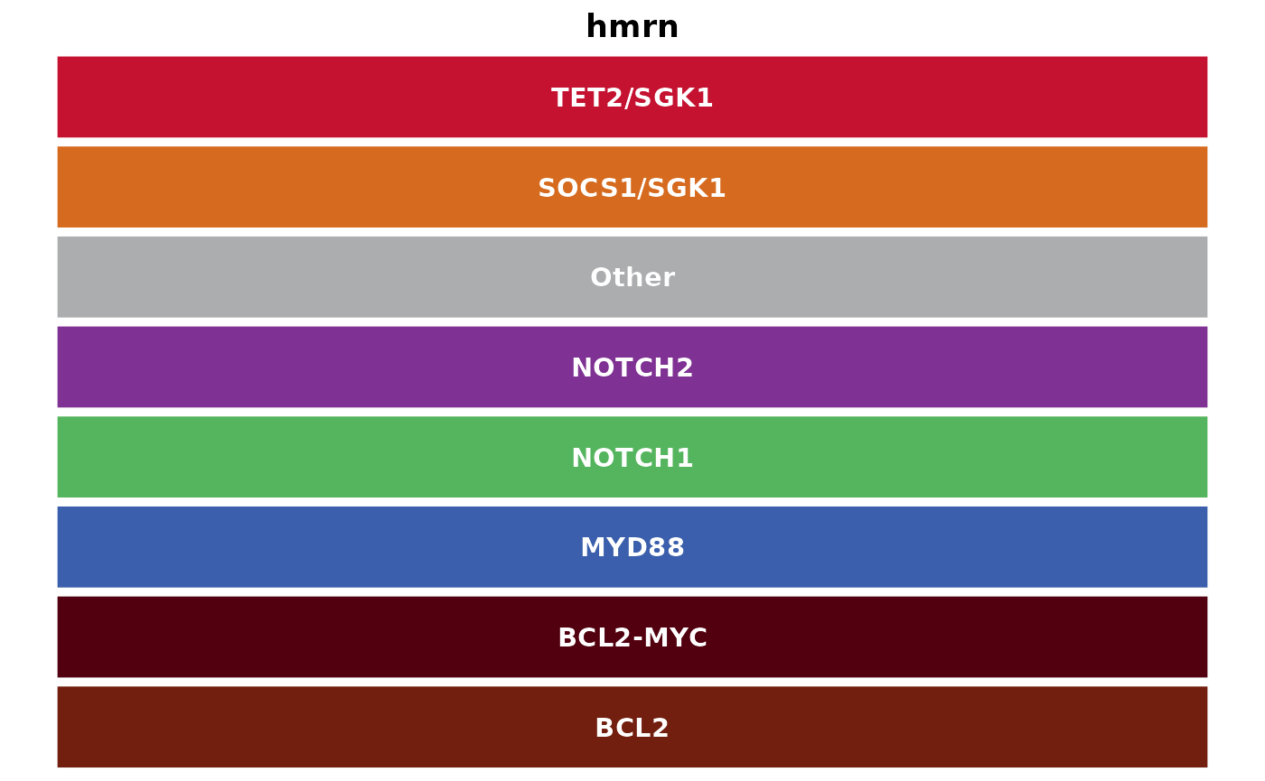
##
## [[4]]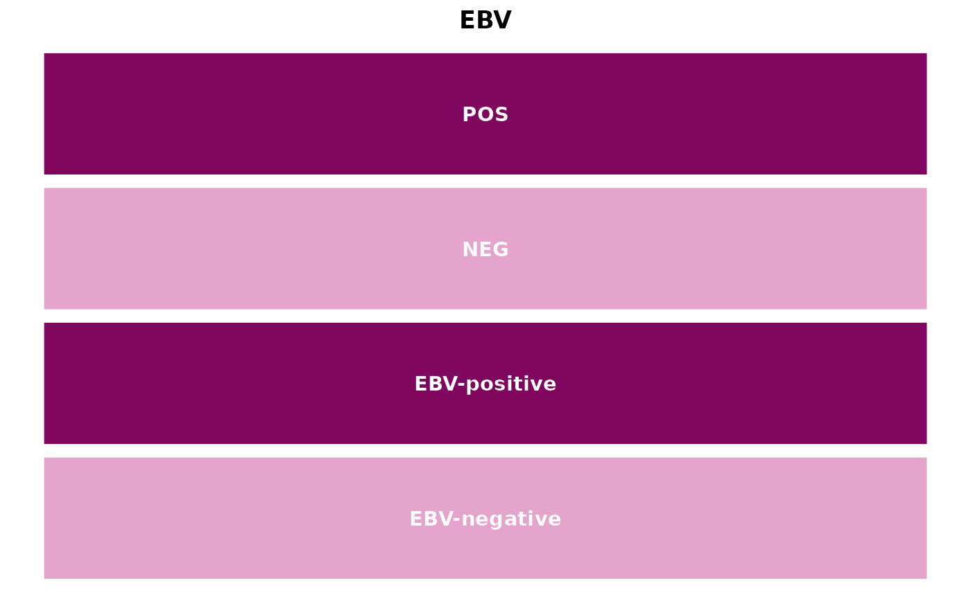
##
## [[5]]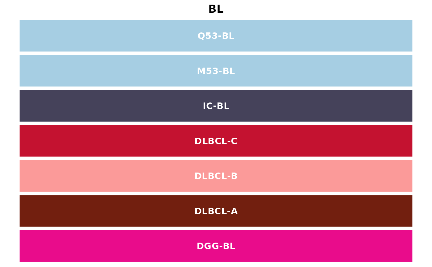
##
## [[6]]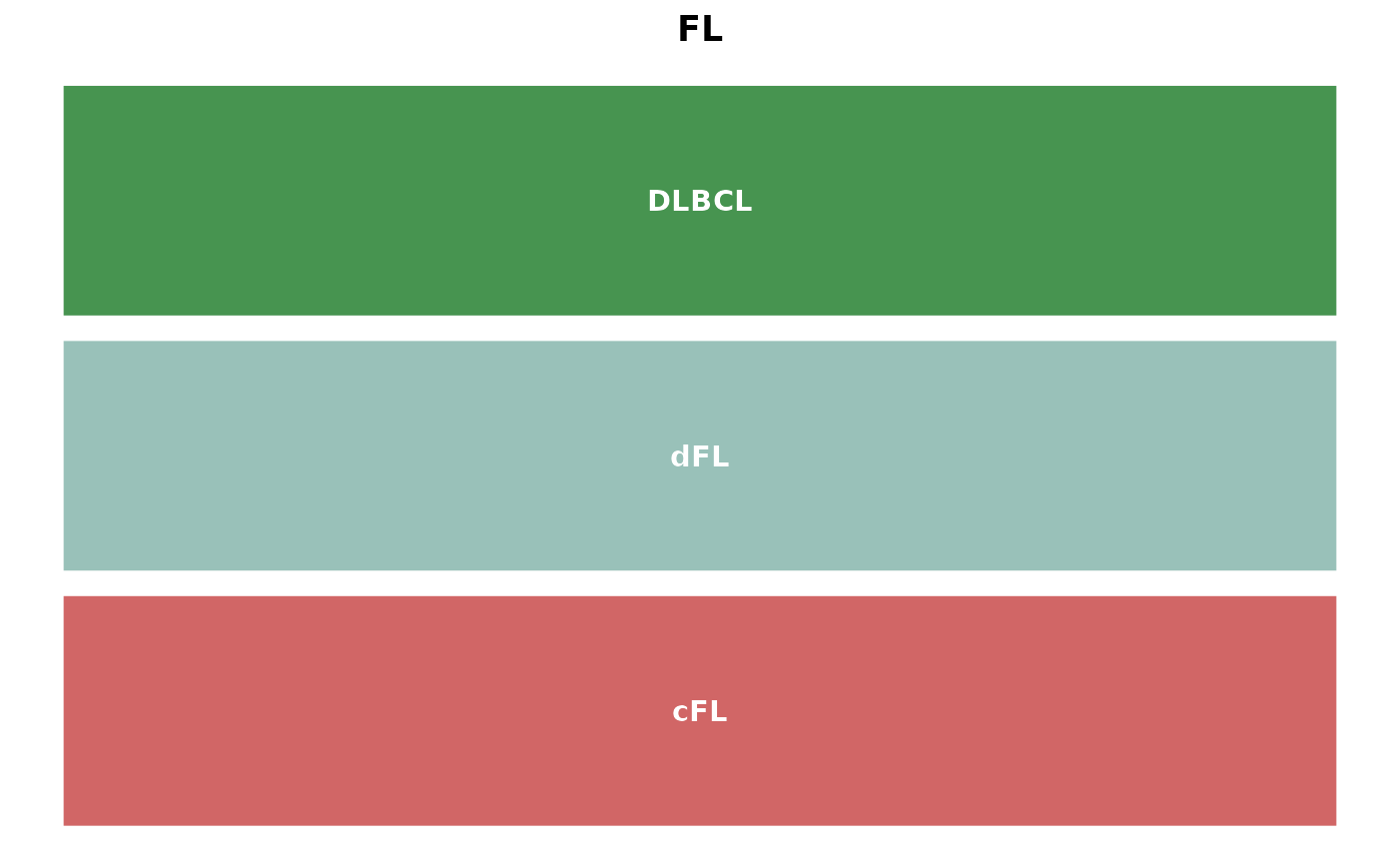
##
## [[7]]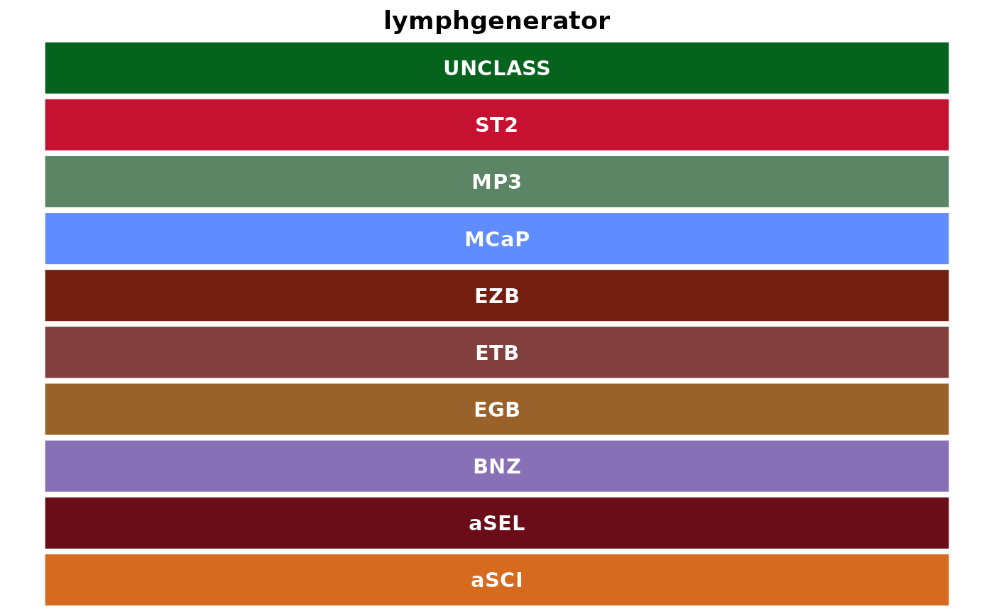
##
## [[8]]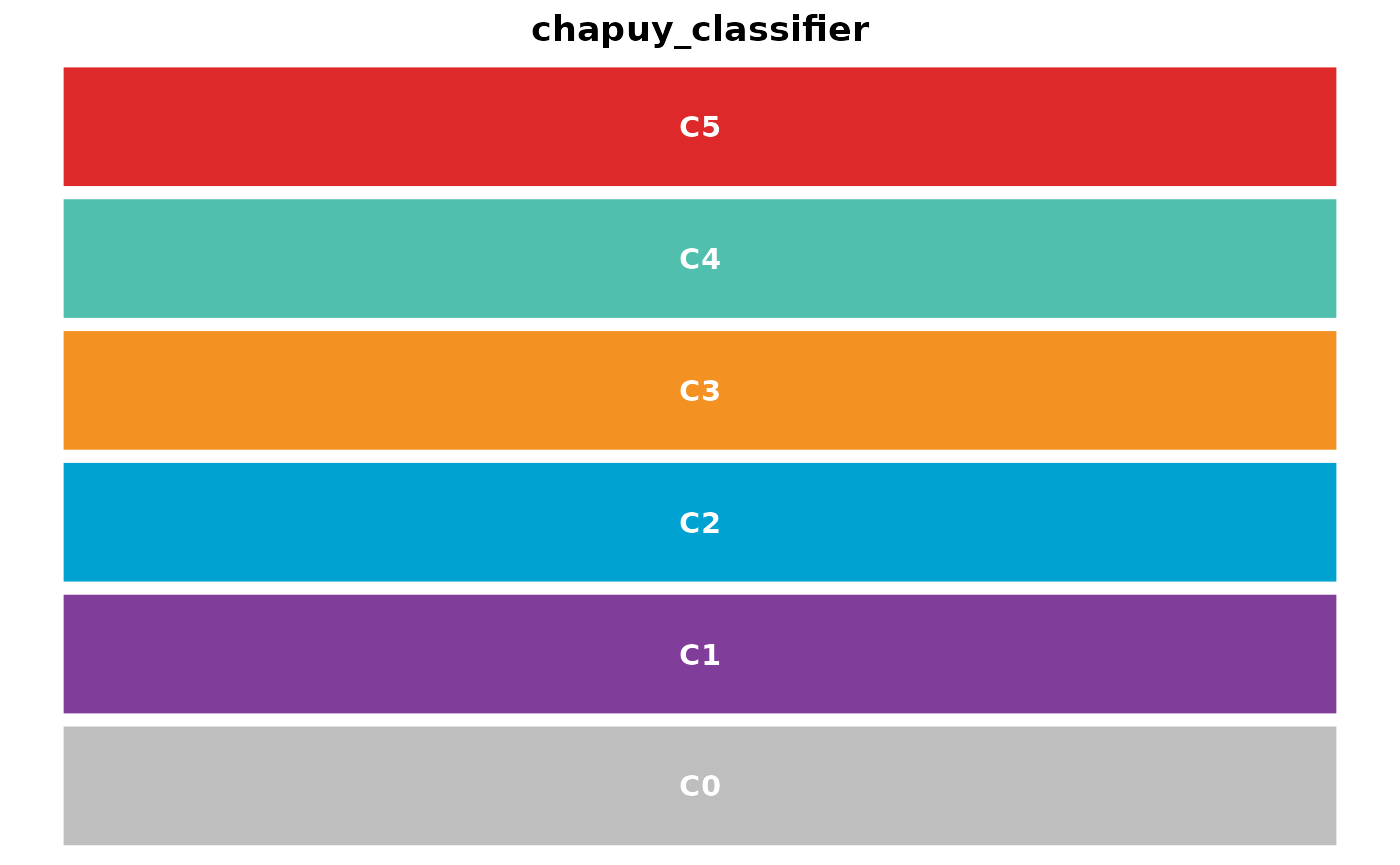
##
## [[9]]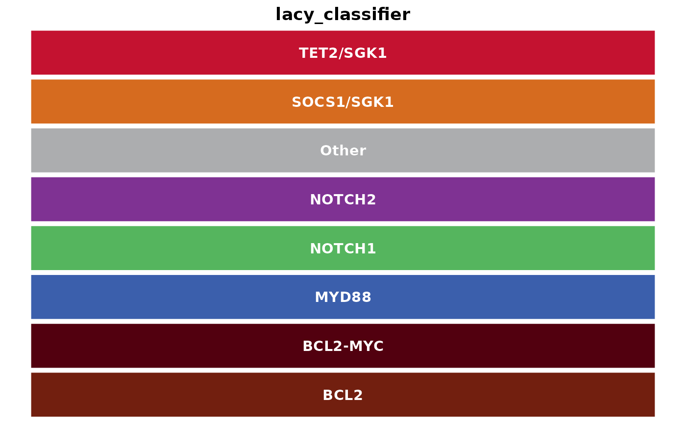
##
## [[10]]
##
## [[11]]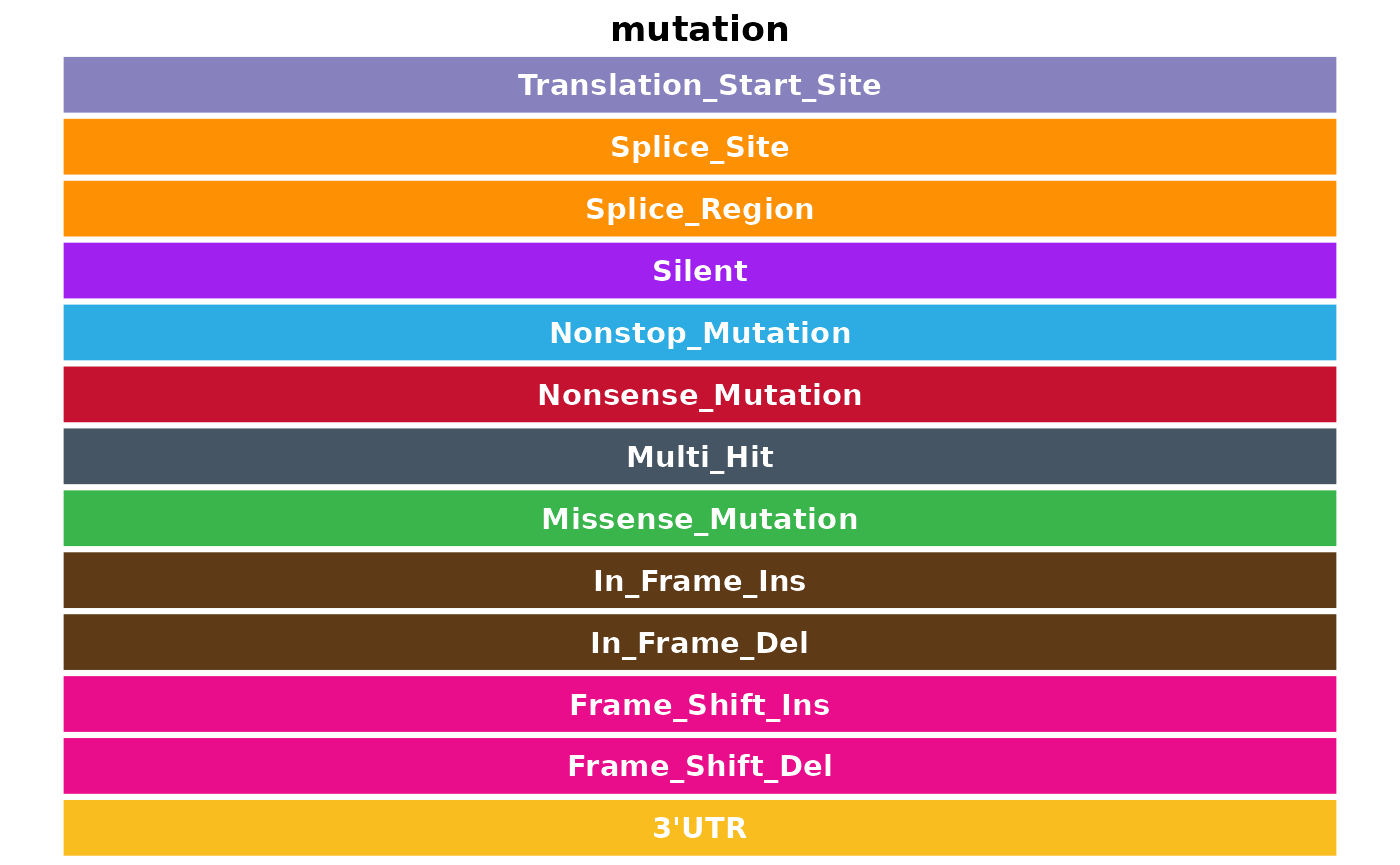
##
## [[12]]
##
## [[13]]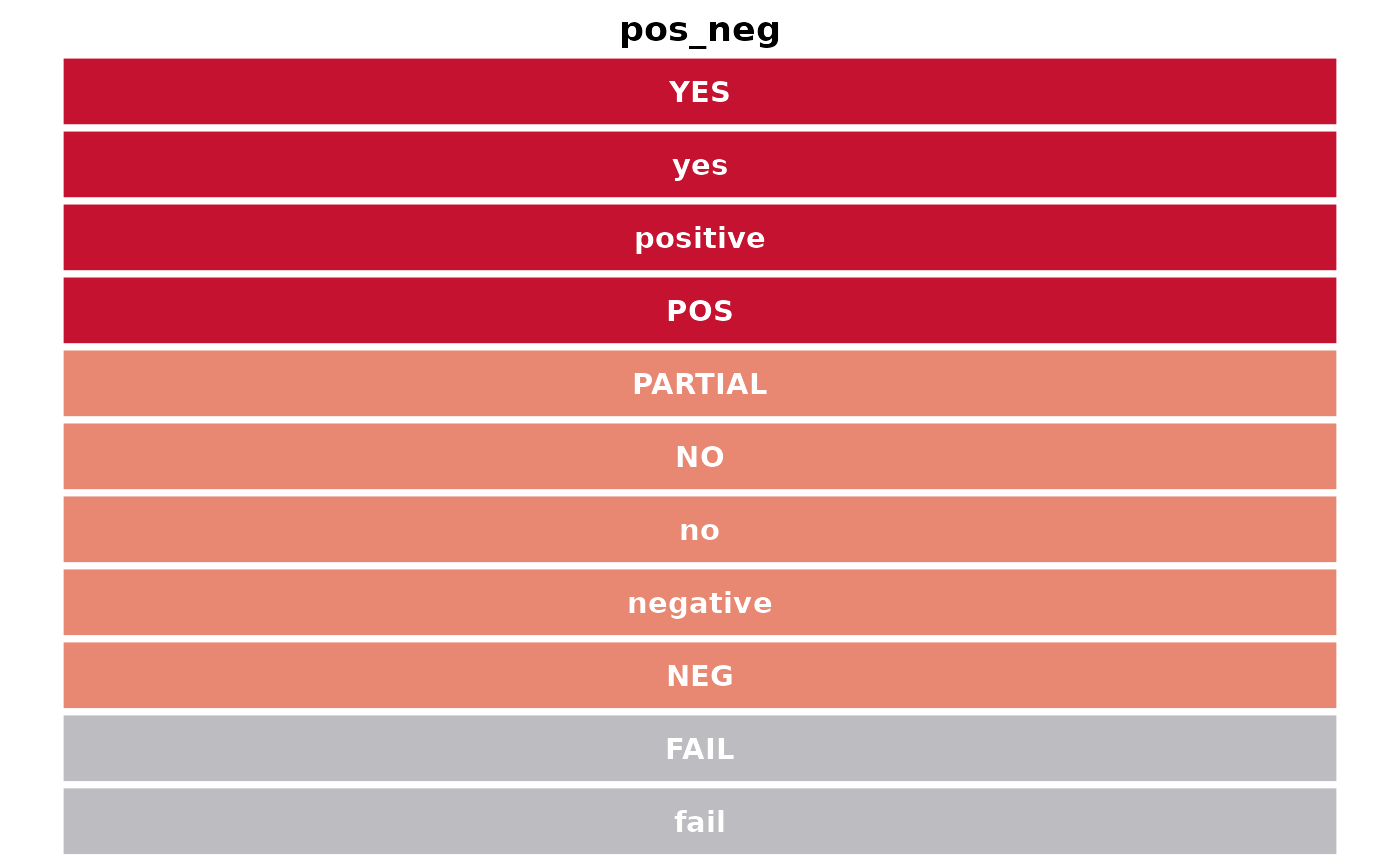
##
## [[14]]
##
## [[15]]
##
## [[16]]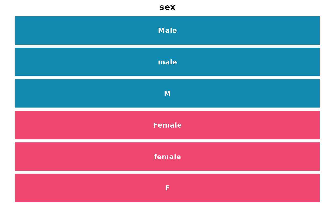
##
## [[17]]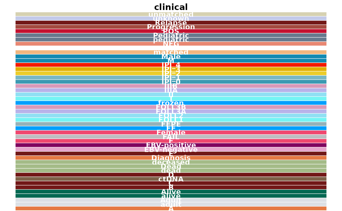
##
## [[18]]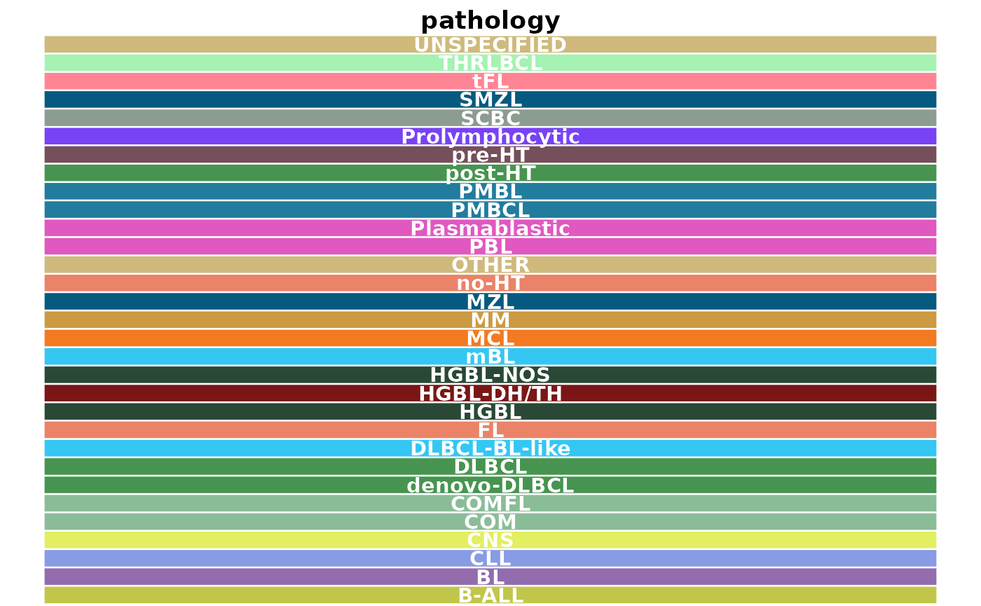
##
## [[19]]
##
## [[20]]
##
## [[21]]
##
## [[22]]
##
## [[23]]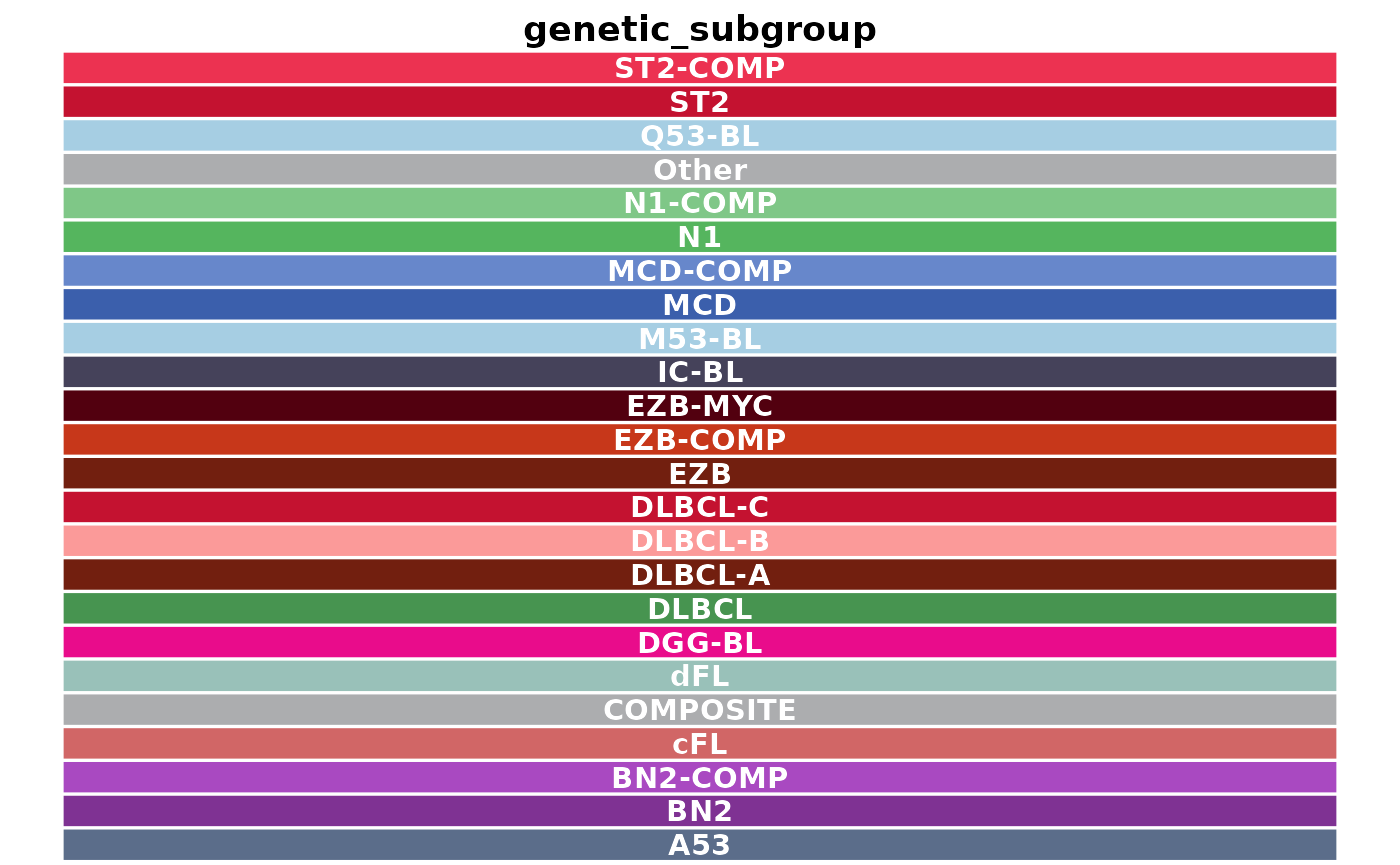
Gene Clouds
Create a wordcloud from an incoming MAF with the prettyGeneCloud function. This function creates a figure with gene symbols from the provided maf, were the size of each printed gene symbol is proportional to the total n occurances in the maf. Required parameter is maf_df. Optional parameters are these_genes, other_genes, these_genes_colour, other_genes_colour and colour_index. If no genes are supplied when calling the function, this function will default to all lymphoma genes.
#get all coding SSM
maf = get_coding_ssm(seq_type = "genome")

#get gene symbols from MAF and subset to chr1
maf_genes = dplyr::filter(maf, Hugo_Symbol != "Unknown") %>%
  dplyr::filter(Chromosome == "1") %>%
  pull(Hugo_Symbol)

#build wordcloud
prettyGeneCloud(maf_df = maf, these_genes = maf_genes)
## Hugo_Symbol n
## 1 A3GALT2 4
## 2 AADACL3 6
## 3 AADACL4 7
## 4 ABCA4 30
## 5 ABCB10 5
## 6 ABCD3 5
## 7 ABL2 8
## 8 AC096677.1 3
## 9 AC119673.1 1
## 10 ACADM 6
## 11 ACAP3 7
## 12 ACBD3 7
## 13 ACBD6 1
## 14 ACOT11 8
## 15 ACOT7 5
## 16 ACP6 4
## 17 ACTA1 5
## 18 ACTL8 3
## 19 ACTN2 15
## 20 ACTRT2 1
## 21 ADAM15 8
## 22 ADAM30 9
## 23 ADAMTS4 5
## 24 ADAMTSL4 22
## 25 ADAMTSL4-AS1 6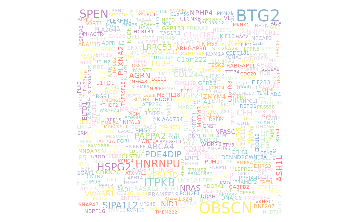
## # A tibble: 2,006 × 2
##    Hugo_Symbol     n
##    <fct>       <int>
##  1 AC119673.1      1
##  2 ACBD6           1
##  3 ACTRT2          1
##  4 AGTRAP          1
##  5 AHCYL1          1
##  6 AKIRIN1         1
##  7 AL109927.1      1
##  8 AL136115.1      1
##  9 AL138847.1      1
## 10 AL139147.1      1
## # ℹ 1,996 more rows